Experimenting with Gradient Descent in Python

For awhile now, the Computer Science department at my University has offered a class for non-CS students called “Data Witchcraft“. The idea, I suppose, is that when you don’t understand how a technology works, it’s essentially “magic“. (And when it has to do with computers and data, it’s dark magic at that.)

But even as someone who writes programs all day long, there are often tools, algorithms, or ideas we use that we don’t really understand–just take at face value, because well, they seem to work, we’re busy, and learning doesn’t seem necessary when the problem is already sufficiently solved.

One of the more prevalent algorithms of this sort is Gradient Descent (GD). The algorithm is both conceptually simple (everyone likes to show rudimentary sketches of a blindfolded stick figure walking down a mountain) and mathematically rigorous (next to those simple sketches, we show equations with partial derivatives across n-dimensional vectors mapped to an arbitrarily sized higher-dimensional space).
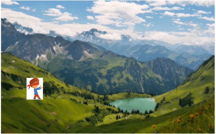
Screen Shot 2016-12-15 at 11.54.44 PM.png
Image from course slides

So most often, after learning about GD, you are sent off into the wild to use it, without ever having programmed it from scratch. From this view, Gradient Descent is a sort of incantation we Supreme Hacker Mage Lords can use to solve complex optimization problems whenever our data is in the right format, and we want a quick fix. (Kind of like Neural Networks and “Deep Learning”…) This is practical for most people who just need to get things done. But it’s also unsatisfying for others (myself included).

However, GD can also be implemented in just a few lines of code (even though it won’t be as highly optimized as an industrial-strength version).

That’s why I’m sharing some implementations of both Univariate and generalized Multivariate Gradient Descent written in simple and annotated Python.

Anyone curious about a working implementation (and with some test data in hand) can try this out to experiment. The code snippets below have print statements built in so you can see how your model changes every iteration.

Full Repository

To download and run the full repo, clone it from here:  https://github.com/adpoe/Gradient_Descent_From_Scratch 

But the actual algorithms are also extracted below, for ease of reading.

Univariate Gradient Descent

Requires NumPy.

Also Requires data to be in this this format:  [(x1,y1), (x2,y2) … (xn,yn)], where Y is the actual value.


def gradient_descent(training_examples, alpha=0.01):
"""
Apply gradient descent on the training examples to learn a line that fits through the examples
:param examples: set of all examples in (x,y) format
:param alpha = learning rate
:return:
"""
# initialize w0 and w1 to some small value, here just using 0 for simplicity
w0 = 0
w1 = 0
# repeat until "convergence", meaning that w0 and w1 aren't changing very much
# –> need to define what 'not very much' means, and that may depend on problem domain
convergence = False
while not convergence:
# initialize temporary variables, and set them to 0
delta_w0 = 0
delta_w1 = 0
for pair in training_examples:
# grab our data points from the example
x_i = pair[0]
y_i = pair[1]
# calculate a prediction, and find the error
h_of_x_i = model_prediction(w0,w1,x_i)
delta_w0 += prediction_error(w0,w1, x_i, y_i)
delta_w1 += prediction_error(w0,w1,x_i,y_i)*x_i
# store previous weighting values
prev_w0 = w0
prev_w1 = w1
# get new weighting values
w0 = w0 + alpha*delta_w0
w1 = w1 + alpha*delta_w1
alpha -= 0.001
# every few iterations print out current model
# 1. –> (w0 + w1x1 + w2x2 + … + wnxn)
print "Current model is: ("+str(w0)+" + "+str(w1)+"x1)"
# 2. –> averaged squared error over training set, using the current line
summed_error = sum_of_squared_error_over_entire_dataset(w0, w1, training_examples)
avg_error = summed_error/len(training_examples)
print "Average Squared Error="+str(avg_error)
# check if we have converged
if abs(prev_w0 w0) < 0.00001 and abs(prev_w1 w1) < 0.00001:
convergence = True
# after convergence, print out the parameters of the trained model (w0, … wn)
print "Parameters of trained model are: w0="+str(w0)+", w1="+str(w1)
return w0, w1
############################
##### TRAINING HELPERS #####
############################
def model_prediction(w0, w1, x_i):
return w0 + (w1 * x_i)
def prediction_error(w0, w1, x_i, y_i):
# basically, we just take the true value (y_i)
# and we subtract the predicted value from it
# this gives us an error, or J(w0,w1) value
return y_i model_prediction(w0, w1, x_i)
def sum_of_squared_error_over_entire_dataset(w0, w1, training_examples):
# find the squared error over the whole training set
sum = 0
for pair in training_examples:
x_i = pair[0]
y_i = pair[1]
sum += prediction_error(w0,w1,x_i,y_i) ** 2
return sum

view raw

uni_gd.py

hosted with ❤ by GitHub

Multivariate Gradient Descent

Requires NumPy, same as above.

Also Requires data to be in this this format:  [(x1,..xn, y),(x1,..xn, y) …(x1,..xn, y)], where Y is the actual value. Essentially, you can have as many x-variables as you’d like, as long as the y-value is the last element of each tuple.


def multivariate_gradient_descent(training_examples, alpha=0.01):
"""
Apply gradient descent on the training examples to learn a line that fits through the examples
:param examples: set of all examples in (x,y) format
:param alpha = learning rate
:return:
"""
# initialize the weight and x_vectors
W = [0 for index in range(0, len(training_examples[0][0]))]
# W_0 is a constant
W_0 = 0
# repeat until "convergence", meaning that w0 and w1 aren't changing very much
# –> need to define what 'not very much' means, and that may depend on problem domain
convergence = False
while not convergence:
# initialize temporary variables, and set them to 0
deltaW_0 = 0
deltaW_n = [0 for x in range(0,len(training_examples[0][0]))]
for pair in training_examples:
# grab our data points from the example
x_i = pair[0]
y_i = pair[1]
# calculate a prediction, and find the error
# needs to be an element-wise plus
deltaW_0 += multivariate_prediction_error(W_0, y_i, W, x_i)
deltaW_n = numpy.multiply(numpy.add(deltaW_n, multivariate_prediction_error(W_0, y_i, W, x_i)), x_i)
#print "DELTA_WN = " + str(deltaW_n)
# store previous weighting values
prev_w0 = W_0
prev_Wn = W
# get new weighting values
W_0 = W_0 + alpha*deltaW_0
W = numpy.add(W,numpy.multiply(alpha,deltaW_n))
alpha -= 0.001
# every few iterations print out current model
# 1. –> (w0 + w1x1 + w2x2 + … + wnxn)
variables = [( str(W[i]) + "*x" + str(i+1) + " + ") for i in range(0,len(W))]
var_string = ''.join(variables)
var_string = var_string[:3]
print "Current model is: " + str(W_0)+" + "+var_string
# 2. –> averaged squared error over training set, using the current line
summed_error = sum_of_squared_error_over_entire_dataset(W_0, W, training_examples)
avg_error = summed_error/len(training_examples)
print "Average Squared Error="+str(sum(avg_error))
print ""
# check if we have converged
if abs(prev_w0 W_0) < 0.00001 and abs(numpy.subtract(prev_Wn, W)).all() < 0.00001:
convergence = True
# after convergence, print out the parameters of the trained model (w0, … wn)
variables = [( "w"+str(i+1)+"="+str(W[i])+", ") for i in range(0,len(W))]
var_string = ''.join(variables)
var_string = var_string[:2]
print "RESULTS: "
print "\tParameters of trained model are: w0="+str(W_0)+", "+var_string
return W_0, W
################################
##### MULTIVARIATE HELPERS #####
################################
# generalize these to just take a w0, a vector of weights, and a vector x-values
def multivariate_model_prediction(w0, weights, xs):
return w0 + numpy.dot(weights, xs)
# again, this needs to take just a w0, vector of weights, and a vector of x-values
def multivariate_prediction_error(w0, y_i, weights, xs):
# basically, we just take the true value (y_i)
# and we subtract the predicted value from it
# this gives us an error, or J(w0,w1) value
return y_i multivariate_model_prediction(w0, weights, xs)
# should be the same, but use the generalize functions above, and update the weights inside the vector titself
# also need to have a vector fo delta_Wn values to simplify
def multivariate_sum_of_squared_error_over_entire_dataset(w0, weights, training_examples):
# find the squared error over the whole training set
sum = 0
for pair in training_examples:
x_i = pair[0]
y_i = pair[1]
# cast back to values in range [1 –> 20]
prediction = multivariate_model_prediction(w0,weights,x_i) / (1/20.0)
actual = y_i / (1/20.0)
error = abs(actual prediction)
error_sq = error ** 2
sum += error_sq
return sum

view raw

mv_grad_desc.py

hosted with ❤ by GitHub

My data set is included in the full repo. But feel free to try it on your own, if you’re experimenting with this. And enjoy.

Comparing Page Replacement Algorithms via Simulation in Python

tl;dr

While studying Operating Systems, I decided to experiment with 4 of the most common Page Replacement algorithms, via simulation, using Python. Input data for my simulations were two memory traces named “swim.trace” and “gcc.trace” (provided by my CS department). All algorithms are run within a page table implemented for a 32-bit address space; all pages in this page table are 4kb in size.

I chose to implement these algorithms and the page table in Python. The final source code can be found here, on Github. The full data set that I collected can be found at the end of this document. Illustrative graphs are interspersed throughout, wherever they are necessary for explaining and documenting decisions.

In this essay itself, I will first outline the algorithms implemented, noting design decisions I made during my implementations. I will then compare and contrast the results of each algorithm when run on the two provided memory traces. Finally, I will conclude with my decision about which algorithm would be best to run in a real Operating System.

Please note, to run the algorithms themselves, you must run:

  • python vmsim.py –n -a <opt|clock|aging|lru> [-r ]


The Algorithms

The algorithms we have been asked to implement are:

  • Opt– Simulate what the optimal page replacement algorithm would choose if it had perfect knowledge
    • EXAMPLE RUN: python vmsim.py –n 8 –a opt gcc.trace
  • Clock– Use the better implementation of the second-chance algorithm
    • EXAMPLE RUN: python vmsim.py –n 16 –a clock swim.trace
  • Aging– Implement the aging algorithm that approximates LRU with an 8-bit counter
    • EXAMPLE RUN: python vmsim.py –n 32 –a aging –r 1 gcc.trace
  • LRU– Do exact LRU.
    • EXAMPLE RUN: python vmsim.py –n 64 –a lru swim.trace

Implementation Notes

The main entry point for the program is the file named vmsim.py. This is the file which must be invoked from the command line to run the algorithms. Because this is a python file, it must be called with “python vmsim.py … etc.”, instead of “./vmsim”, as a C program would. Please make sure the selected trace file is in the same directory as vmsim.py.

All algorithms run within a page table, the implementation of which can be found in the file named pageTable.py.

Upon program start, the trace file is parsed by the class in the file parseInput.py, and each memory lookup is stored in a list of tuples, in this format: [(MEM_ADDRESS_00, R/W), [(MEM_ADDRESS_01, R/W), … [(MEM_ADDRESS_N, R/W)]. This list is then passed to whichever algorithm is invoked, so it can run the chosen algorithm on the items in the list, element by element.

The OPT algorithm can be found in the file opt.py. My implementation of OPT works by first preprocessing all of the memory addresses in our Trace, and creating a HashTable where the key is our VPN, and the value is a python list containing each of the address numbers at which those VPNs are loaded. Each time a VPN is loaded, the element at index 0 in that list is discarded. This way, we only have to iterate through the full trace once, and from there on out we just need to hash into a list and take the next element, whenever we want to know how far into the future that VPN is next used.

The Clock Algorithm is implemented in the files clock.py and circularQueue.py. My implementation uses the second chance algorithm with a Circular Queue. Of importance: whenever we need to make an eviction, but fail to find ANY pages that are clean, we then run a ‘swap daemon’ which writes out ALL dirty pages to disk at that time. This helps me get fewer page faults, at the expense of more disk writes. That’s a calculated decision for this particular algorithm, since the project description says we should use page faults as our judgment criterion for each algorithm’s effectiveness.

The LRU Algorithm can be found in the file lru.py. For LRU, each time a page is Read, I mark the memory address number at which this happens in the frame itself. Then, in the future—whenever I need to make an eviction—I have easy access to see which frame was used the longest time in the past, and no difficult calculations are needed. This was the simplest algorithm to implement.

The Aging Algorithm is likely the most complex, and its source code can be found in the file named aging.py. Aging works by keeping an 8 bit counter and marking whether each page in the page table was used during the last ‘tick’ a time period of evaluation which must be passed in by the user as a ‘refresh rate’, whenever the Aging Algorithm is selected. All refresh rates are in milliseconds on my system, but this relies on the implementation of Python’s “time” module, so it’s possible that this could vary on other systems. For aging, I suggest a refresh rate of 0.01 milliseconds, passed in on the command line as “-r 0.01”, in the 2nd to last position in the arg list. This minimizes the values in my testing, and going lower does not positively affect anything. In the next section, I will show my rationale for selecting 0.01 as my refresh rate.

Aging Algorithm Refresh Rate

In order to find a refresh rate that would work well, I decided to start at 1ms and move 5 orders of magnitude in each direction, from 0.00001ms to 100000ms.

To ensure that the results were not biased toward being optimized for a single trace, I tried both to confirm that the refresh rate would work will for all inputs.

The graphs below show the Page Faults and Disk Writes I found during each test.

For all tests, I chose a frame size of 8, since this small frame size is most sensitive to the algorithm used. At higher frame sizes, all of the algorithms tend to perform better, across the board. So I wanted to focus on testing at the smallest possible size, preparing for a ‘worst case’ scenario.

Aging Algorithm – Page Faults Over Refresh Rate

screen-shot-2016-12-01-at-3-11-50-pm

X-axis:   Refresh rate in milliseconds

Y-axis:   Total Page faults

GCC. TRACE reaches its minimum for page faults at 0.0001ms and SWIM.TRACE reaches its own minimum at 0.01ms. The lines cross at around 0.01ms.


Total Page Faults For SWIM.TRACE – Detail

screen-shot-2016-12-01-at-3-09-24-pm

X-axis: Page Faults

Y-Axis: Refresh Rates

screen-shot-2016-12-01-at-3-14-18-pm

X-axis: Page Faults

Y-Axis: Refresh Rates

Additionally, 0.01ms seems to achieve the best balance, in my opinion, if we need to select a single time for BOTH algorithms.


Aging Algorithm – Disk Writes Over Refresh Rate

screen-shot-2016-12-01-at-3-09-42-pm

X-axis:   Refresh rate in milliseconds

Y-axis:   Total Disk Writes

The number of disk writes also bottoms out at 0.01ms from SWIM.TRACE. It is relatively constant for GCC.TRACE across all of the different timing options.

Because of this, I suggest 0.01ms as the ideal refresh rate. This is because it is optimal for SWIM.TRACE. For GCC.TRACE, it is not the absolute best option, but it is still acceptable, and so I think this selection will achieve a good balance.

Results & Decisions

With the algorithms all implemented, my next step was to collect data for each algorithm at all frame sizes, 8, 16, 32, and 64. OPT always performed best, and thus it was used as our baseline.

In the graphs below, I show how each algorithm performed, both in terms of total page faults and total disk writes.

SWIM.TRACE – Page Faults Over Frame Size

screen-shot-2016-12-01-at-3-10-02-pm

X-axis:   Frame Size

Y-axis:   Page Faults

Data for all algorithms processing swim.trace

SWIM.TRACE – Disk Writes Over Frame Size

screen-shot-2016-12-01-at-3-10-09-pm

X-axis:   Frame Size

Y-axis:   Disk Writes

Data for all algorithms processing swim.trace

GCC.TRACE – Page Faults Over Frame Size

screen-shot-2016-12-01-at-3-10-16-pm

X-axis:   Frame Size

Y-axis:   Page Faults

Data for all algorithms processing gcc.trace

GCC.TRACE – Disk Writes Over Frame Size

screen-shot-2016-12-01-at-3-10-24-pm

X-axis:   Frame Size

Y-axis:   Disk Writes

Data for all algorithms processing gcc.trace

Given this data, I was next tasked with choosing which algorithm is most appropriate for an actual operating system.

In order to determine which algorithm would be best, I decided to use an algorithm. I’ll call it the ‘Decision Matrix’, and here are the steps.

DECISION MATRIX:

  1. RANK ALGORITHMS FOR EACH CATEGORY FROM 1=BEST to 4=WORST,
  2. SELECT ALGORITHM WITH LOWEST OVERALL SCORE
ALGORITHM SWIM – Page Faults SWIM – Disk Writes GCC – Page Faults GCC – Disk Writes TOTAL (Lowest is Best)
OPT 1 1 1 1 4
CLOCK 2 4 2 4 12
AGING 4 2 4 2 12
LRU 3 3 3 3 12


Ranking:             1=Best;

                               4=Worst

NOTE:

  • Wherever lines cross each other in our graphs, the algorithm ranked as “better” is the one with MORE total low data points. Ties were broken by my own personal judgment.

Decision:

  • Of course, using this set of judgment criteria, OPT is by far the winner.
  • However OPT isn’t an option in a real OS, since it requires perfect knowledge of the future, which is impossible in practice.
  • So we want to pick between the 3-way tie for CLOCK and LRU and AGING.
    • Of these three:
      • AGING does well on disk writes, but generally has the most page faults.
      • Conversely, CLOCK does well on page faults, but often has the most disk writes.
      • LRU achieves a balance.
    • Therefore, My pick goes to LRU, because where clock does beat LRU, on page faults it does so only by a narrow margin.
    • But where LRU beats clock—on disk writes—it does so by a large amount. This means LRU is better overall, if both page faults and disk writes are equally weighted for judgment purposes.

Therefore, I would select LRU for my own operating system.

Data Set

Figure 1.1 – Full Data Set

ALGORITHM NUMBER OF FRAMES TOTAL MEMORY ACCESSES TOTAL PAGE FAULTS TOTAL WRITES TO DISK TRACE REFRESH RATE
OPT 8 1000000 236350 51162 swim.trace N/A
OPT 16 1000000 127252 27503 swim.trace N/A
OPT 32 1000000 52176 11706 swim.trace N/A
OPT 64 1000000 24344 6316 swim.trace N/A
OPT 8 1000000 169669 29609 gcc.trace N/A
OPT 16 1000000 118226 20257 gcc.trace N/A
OPT 32 1000000 83827 14159 gcc.trace N/A
OPT 64 1000000 58468 9916 gcc.trace N/A
CLOCK 8 1000000 265691 55664 swim.trace N/A
CLOCK 16 1000000 136154 52104 swim.trace N/A
CLOCK 32 1000000 73924 45872 swim.trace N/A
CLOCK 64 1000000 56974 43965 swim.trace N/A
CLOCK 8 1000000 178111 38992 gcc.trace N/A
CLOCK 16 1000000 122579 26633 gcc.trace N/A
CLOCK 32 1000000 88457 20193 gcc.trace N/A
CLOCK 64 1000000 61832 15840 gcc.trace N/A
AGING 8 1000000 257952 52664 swim.trace 0.01ms
AGING 16 1000000 143989 41902 swim.trace 0.01ms
AGING 32 1000000 91852 29993 swim.trace 0.01ms
AGING 64 1000000 82288 27601 swim.trace 0.01ms
AGING 8 1000000 244951 31227 gcc.trace 0.01ms
AGING 16 1000000 187385 22721 gcc.trace 0.01ms
AGING 32 1000000 161117 19519 gcc.trace 0.01ms
AGING 64 1000000 149414 16800 gcc.trace 0.01ms
LRU 8 1000000 274323 55138 swim.trace N/A
LRU 16 1000000 143477 47598 swim.trace N/A
LRU 32 1000000 75235 43950 swim.trace N/A
LRU 64 1000000 57180 43026 swim.trace N/A
LRU 8 1000000 181950 37239 gcc.trace N/A
LRU 16 1000000 124267 23639 gcc.trace N/A
LRU 32 1000000 88992 17107 gcc.trace N/A
LRU 64 1000000 63443 13702 gcc.trace N/A

Figure 1.2 – GCC.TRACE – Refresh Rate Testing – 8 Frames

ALGORITHM NUMBER OF FRAMES TOTAL MEMORY ACCESSES TOTAL PAGE FAULTS TOTAL WRITES TO DISK TRACE REFRESH RATE
AGING 8 1000000 192916 33295 gcc.trace 0.00001ms
AGING 8 1000000 192238 33176 gcc.trace 0.0001ms
AGING 8 1000000 197848 31375 gcc.trace 0.001ms
AGING 8 1000000 244951 31227 gcc.trace 0.01ms
AGING 8 1000000 339636 140763 gcc.trace 0.1ms

Figure 1.3 –SWIM.TRACE – Refresh Rate Testing – 8 Frames

ALGORITHM NUMBER OF FRAMES TOTAL MEMORY ACCESSES TOTAL PAGE FAULTS TOTAL WRITES TO DISK TRACE REFRESH RATE
AGING 8 1000000 275329 53883 swim.trace 0.00001ms
AGING 8 1000000 274915 53882 swim.trace 0.0001ms
AGING 8 1000000 268775 53540 swim.trace 0.001ms
AGING 8 1000000 257952 52664 swim.trace 0.01ms
AGING 8 1000000 278471 56527 swim.trace 0.1ms

Experimenting with the Harris Corner Detector Algorithm in Matlab

tl;dr

Example code to start experimenting with the Harris Corner Detection Algorithm on your own, in Matlab. And some of the results I obtained in my own testing.

Corner Cases

Among the classic algorithms in Computer Vision is Harris Corner Detection. (For the original paper, from 1988, see here.) The problem it solves:  Given any image file, can you find which areas correspond to a corner with a high degree of certainty?

The answer is yes. And the algorithm is elegant. Essentially the steps are:

  1. Convert your image to a Matrix, storing the pixel values by intensity (converting to B/W makes this easier)
  2. Find the horizontal and vertical gradients of the image (essentially the derivative of pixel intensities). This will let us know where there are horizontal and vertical edges.
  3. Scan the image getting groups of pixels for however wide an area you are concerned with, and perform a calculation to determine where the horizontal and vertical edges intersect. (This requires some relatively complex linear algebra, but I’m not focusing on the theory here, just the implementation.)

Recently, I was trying to implement my own version of the Harris Detector in Matlab, and ended up banging my head against the wall for a few hours while figuring out some of the subtler details the hard way.

Here’s the code I came up with, and some examples of the outputs. Grab the code from both gists below, and you can start experimenting on your own.

Harris Algorithm


function [ x, y, scores, Ix, Iy ] = harris_corners( image )
%HARRIS_CORNERS Extracts points with a high degree of 'cornerness' from
%RGB image matrix of type uint8
% Input – image = NxMx3 RGB image matrix
% Output – x = nx1 vector denoting the x location of each of n
% detected keypoints
% y = nx1 vector denoting the y location of each of n
% detected keypoints
% scores = an nx1 vector that contains the value (R) to which a
% a threshold was applied, for each keypoint
% Ix = A matrix with the same number of rows and columns as the
% input image, storing the gradients in the x-direction at each
% pixel
% Iy = A matrix with the same nuimber of rwos and columns as the
% input image, storing the gradients in the y-direction at each
% pixel
% compute the gradients, re-use code from HW2P, use window size of 5px
% convert image to grayscale first
G = rgb2gray(image);
% convert to double
G2 = im2double(G);
% create X and Y Sobel filters
horizontal_filter = [1 0 1; 2 0 2; 1 0 1];
vertical_filter = [1 2 1; 0 0 0 ; 1 2 1];
% using imfilter to get our gradient in each direction
filtered_x = imfilter(G2, horizontal_filter);
filtered_y = imfilter(G2, vertical_filter);
% store the values in our output variables, for clarity
Ix = filtered_x;
Iy = filtered_y;
% Compute the values we need for the matrix…
% Using a gaussian blur, because I get more positive values after applying
% it, my values all skew negative for some reason…
f = fspecial('gaussian');
Ix2 = imfilter(Ix.^2, f);
Iy2 = imfilter(Iy.^2, f);
Ixy = imfilter(Ix.*Iy, f);
% set empirical constant between 0.04-0.06
k = 0.04;
num_rows = size(image,1);
num_cols = size(image,2);
% create a matrix to hold the Harris values
H = zeros(num_rows, num_cols);
% % get our matrix M for each pixel
for y = 6:size(image,1)-6 % avoid edges
for x = 6:size(image,2)-6 % avoid edges
% calculate means (because mean is sum/num pixels)
% generally, this algorithm calls for just finding a sum,
% but using the mean makes visualization easier, in my code,
% and it doesn't change which points are computed to be corners.
% Ix2 mean
Ix2_matrix = Ix2(y2:y+2,x2:x+2);
Ix2_mean = sum(Ix2_matrix(:));
% Iy2 mean
Iy2_matrix = Iy2(y2:y+2,x2:x+2);
Iy2_mean = sum(Iy2_matrix(:));
% Ixy mean
Ixy_matrix = Ixy(y2:y+2,x2:x+2);
Ixy_mean = sum(Ixy_matrix(:));
% compute R, using te matrix we just created
Matrix = [Ix2_mean, Ixy_mean;
Ixy_mean, Iy2_mean];
R1 = det(Matrix) (k * trace(Matrix)^2);
% store the R values in our Harris Matrix
H(y,x) = R1;
end
end
% set threshold of 'cornerness' to 5 times average R score
avg_r = mean(mean(H));
threshold = abs(5 * avg_r);
[row, col] = find(H > threshold);
scores = [];
%get all the values
for index = 1:size(row,1)
%see what the values are
r = row(index);
c = col(index);
scores = cat(2, scores,H(r,c));
end
y = row;
x = col;
end

Displaying Your Results


image = imread('your_image.png');
image = imresize(image, 0.75); # or however much you want to resize if your image is large
[ x, y, scores, Ix, Iy ] = harris_corners( image );
figure; imshow(image)
hold on
for i = 1:size(scores,2)
plot(x(i), y(i), 'ro', 'MarkerSize', scores(i) * 2); # you may need to play with this multiplier or divisor based on your image
# I've used –> (/1000) to (* 10)
end
saveas(gcf,'your_image_with_corners.png');
hold off

My Outputs

Here’s what you can expect to see. I’m coloring the corners RED, using circles that grow larger the more likely the area is to hold a corner. So, larger circles –> more obvious corners. (Also note that I’m downsizing my output images slightly, just to make computation faster. )


Closing

That’s it. With this code, you can start experimenting with Harris Detectors in about 30 seconds. And hopefully the way I’ve written it is transparent enough to make it obvious what’s going on behind the scenes. Most of the implementations out there are somewhat opaque and hard to understand at a conceptual level. But I’m hoping that my contribution will make this all a little more straightforward to those just gettings started. Enjoy. -t

Computing the Energy Function of Great Artworks

tl;dr

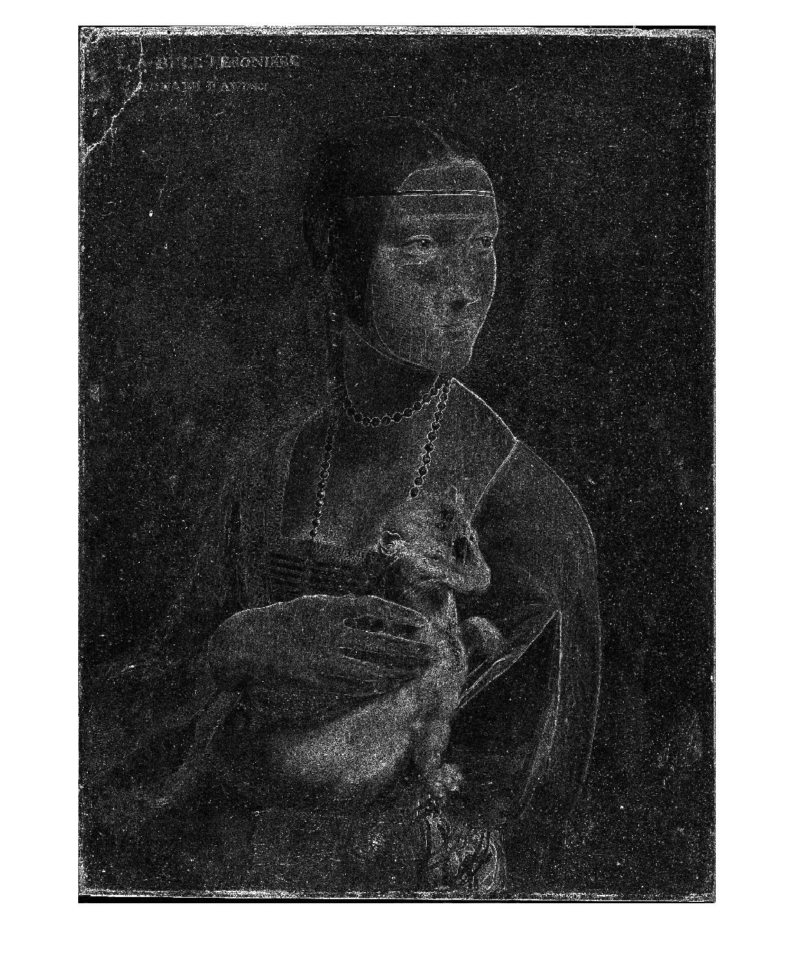
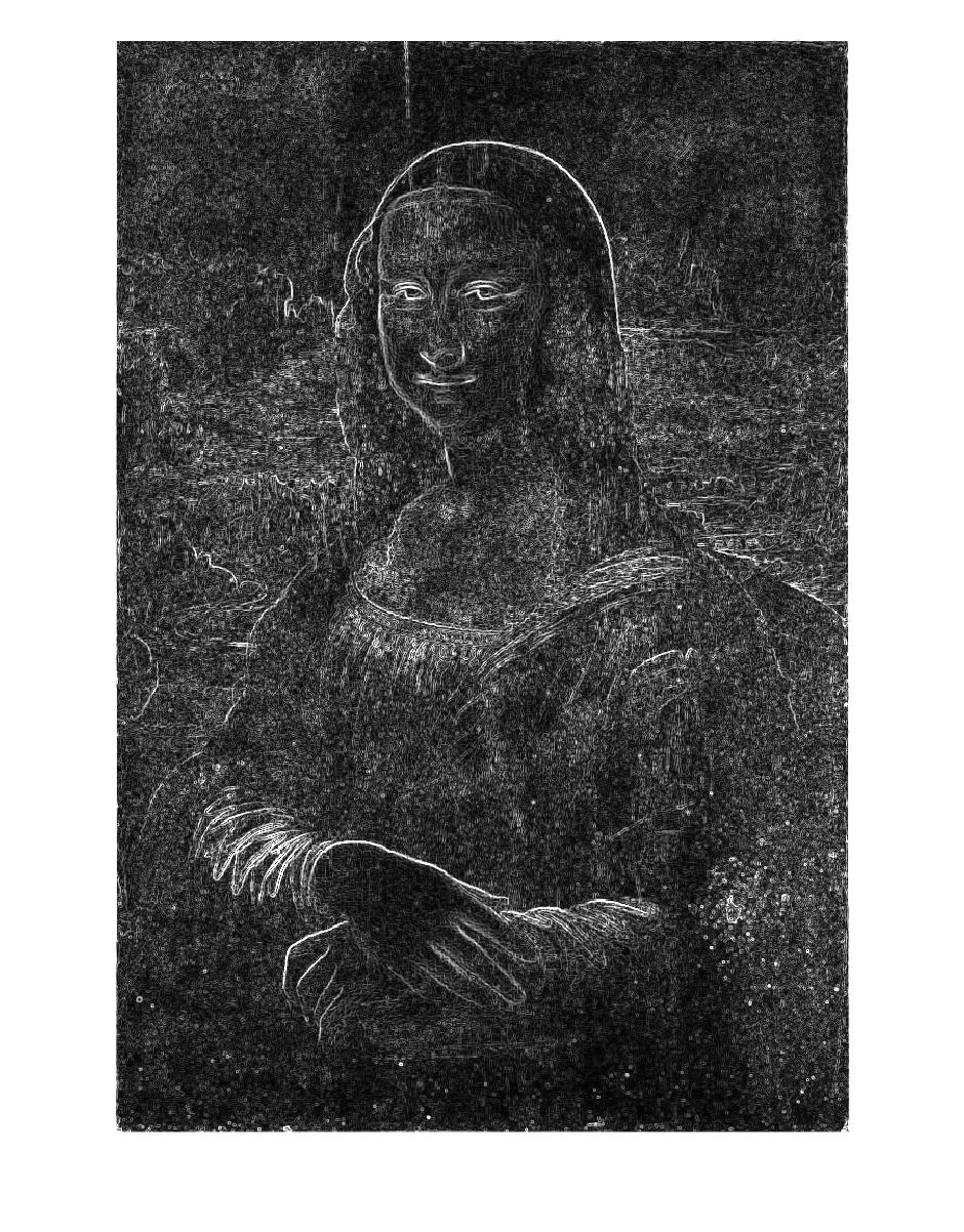
I’m currently working on a computer vision project to implement seam carving, which is explained quickly in this video by the technique’s inventors. The goal of seam carving is to allow for content-aware image resizing. Part of this algorithm is a numerical method to identify the ‘important’ content of an image (at least w/r/t re-sizing). I wanted to see what this algorithm would ID as ‘important’ in some great artworks from history. So I ran the algorithm on some of my favorite paintings (low-res versions from the internet) and am sharing the outputs here.

Brief Technical Explanation (skip if not interested)

The short story is that seam carving allows us to re-size images without distorting the important details. Seam carving is the process of finding connected paths of pixels with “low energy” running through the image–call these paths seams–and then removing those seams instead of a full column or row which might intersect with something important in the image, like a person’s face, the edge of a large object, etc… The easiest way to get an overview is to watch the video above, but hopefully that’s a succinct enough explanation for anyone impatient like me.

The first step in implementing the seam carving algorithm is to compute what’s called the energy function of the image’s pixel gradients. We can do this by plotting the image’s grayscale values (0-255) in a 2D matrix, applying a filter to identify edge gradients in both the x-direction and y-direction, and then computing the magnitude of each pixel’s edge gradient, weighing the x-gradient and y-gradient equally: (i.e. — sqrt(x^2 + y^2) ). If that doesn’t make a ton of sense yet, don’t worry. The video is the easiest way to understand the concept, and reading the paper is the easiest way to understand the process. This is just the super succinct version. (I also probably explained it badly.)

The Energy Function Code


function [ energy_matrix ] = energy_image( image_matrix_input )
%ENERGY_IMAGE Computes the energy at each pixel in a matrix nxmx3 matrix
% Outputs a 2D-matrix containing energy equation outputs, of datatype DBL
% convert image to grayscale first
G = rgb2gray(image_matrix_input);
% convert to double
G2 = im2double(G);
% create X and Y filters
horizontal_filter = [1 0 1; 2 0 2; 1 0 1];
vertical_filter = [1 2 1; 0 0 0 ; 1 2 1];
% using imfilter to get our gradient in each direction
filtered_x = imfilter(G2, horizontal_filter);
filtered_y = imfilter(G2, vertical_filter);
energy_matrix = zeros(size(G2,1), size(G2,2));
% compute the energy at each pixel using the magnitude of the x and y
% gradients: sqrt((dI/dX)^2+(dI/dY)^2))
for y = 1:size(G2, 1)
for x = 1:size(G2,2)
% calculate energy function
y_magnitude = filtered_y(y,x) ^ 2;
x_magnitude = filtered_x(y,x) ^ 2;
energy_output = sqrt( y_magnitude + x_magnitude );
% fill energy matrix with our calculation
energy_matrix(y,x) = energy_output;
end
end
end

view raw

energy.m

hosted with ❤ by GitHub

The Good Stuff

Okay, so now we can compute the energy function of any image.

And the supposed output of this energy function is a mapping where the the important details of the image–the ones we don’t want to carve out when we re-size–are represented in higher intensities of white. The less important details of the image are represented in darker shades of gray and black.

So my question is what happens when we run historical artworks through this algorithm? Does it tell us anything new and novel about artist, his techniques, etc? I’ve always heard that the really well educated and expert art historians can confirm or deny the veracity of an artwork by looking at brush strokes, and the like. I’ve also read stories about taking x-rays of famous artworks, and revealing hidden paintings beneath.

For the most part I’ll let you decide, but in any case, I found some of the outputs to be really beautiful and interesting in their own right. Enough talking for now, here’s the imagery.

You’ll have to click through to see the images in full-size (bottom right button in popup after clicking on the thumbnail), and some of the more interesting details need magnification, which requires downloading the images, just as a heads up.

Da Vinci


Picasso


Bacon


El Greco


De Kooning

Vermeer


Closing

There’s a lot more that can be done with this, of course, and this post has no real analysis, conclusions, or anything of the like. But I wanted to share what I was playing around with, in case anyone else finds it interesting, like I do. -t


On AI-Assisted Creativity

tl;dr

In which I suggest, quite longwindedly, that the next great avant-garde movement in art & music & writing will be AI-Assisted Creativity. I’ll probably edit this later, but it’s something I want to think through and am happy to talk with others about. I’m genuinely very interested in the future of art/creativity and also wondering about others’ opinions and views, where mine fall short, etc.

The First Realization of the Avant-Garde Dream

Before I got into software, I wanted to be an artist. My main focus was on avant-garde art, doing something new, and pushing boundaries—eventually with the goal of merging the mundanities of our everyday lives with our artistic output, such that the entirety of our existence becomes a single, continuous, expressive work of art.

This was the goal of the Happenings in the sixties, the Dadaists in the 20s, even Andy Warhol when he essentially suggested art was all around us, even at the grocery store. (In a strange way this is something akin to the old zen-philosophy, of fully *being* in every moment, seeing its beauty.) And it’s still the goal of performance art that breaks the boundaries between life and performance, like Sleep No More in NYC, and many others across the world. The point is this: you no longer know where reality ends and artifice begins. Because of this, ideally, everything is a form of joyful, creative expression, nothing is ‘work’, and we get lost in an ideal world where we can be artists not workers at some job we don’t care about.

At first, this seemed like a desirable goal to me, and it seemed like it was becoming increasingly possible with more and more online media outlets like YouTube, and Instagram, Facebook and others allowing us to document and color every moment of our lives however we’d like. Every meal, every night out, every workout, all of them can become part of the artwork that is your life—as you present it anyway—a sort of of online self portrait that’s always a work in progress and might just live forever as pure electricity flowing around our planet from satellite to satellite, computer to computer, long after you’ve turned to dust.

There’s something wild and Romantic about that notion, and back in 2009 or 2008, saying those kinds of things at art classes in a University got lots of people angry. But here we are, in 2016, and that’s more or less what happened at some level. Today, I’d suggest, the dream of the avant-garde of the 20th century has largely been fully realized: all of our lives are one continuous artwork, and every moment we’re making art, working on those self-portraits, whether we like it or not. We’re writing, we’re taking photos, films, always and obsessively critiquing.

However, the dream has been realized perversely. Rather than turn everything into joyful creativity, it’s turned all of our lives into one continuous exercise in content farming—it’s not artwork, it’s just **work**, and sometimes even __getting a job__ requires social media presence as a daily necessity. And more pointedly, rather than allowing using to create artwork for our own joy and benefit, we generally cede all copyrights to companies the second we hit post, send, or click.

None of this is news, but the point I’m intending to make is this:
 1) In the 20th century, experimental artists desired to merge art and life together, this was called the avant-garde
 2) By the early 21st century this dream has succeeded. In countries like the United States, many people spend their entire day creating artwork (writing, photos, videos) on platforms like Instagram, or YouTube, etc, Twitter, etc.
3) But rather than freeing artists from the strictures of work and labor, turning life into a wild, creative dream, it’s generally created a more subtle dystopia, where creating artwork is an extra necessary part of daily life
4) So, while the Avant-Garde dream has succeeded, it’s also failed, and in doing so, it’s planted the seeds for the next great trend in artistic innovation, namely: where do we go from here?

Where do we go from here?

Okay, so the Avant-garde dream succeeds, but it creates its own problems, at least in this conception. Now we’re all artists, but we’re giving away our artistic work & hence our very lives to companies that subtly control us in more ways than we really know, and we do so *by the very act* of creating the artwork that we’re more or less necessitated to produce in order to succeed in 21st century life. (When’s the last time you tried to apply for a job that didn’t want to see your personal ‘fun’ Github projects, your witty Twitter comments, or your LinkedIn profile?)

My suggestion is that the really innovative artists will take things one step further. They’ll attempt to merge our digital lives with the very algorithms that control them.

There’s long been a movement, in both software and art, to create programs that allow us to generate artwork, or music, or writing that is more or less indistinguishable from that created by a human. There are reasons for this, and besides being cool, it serves as a basis Turing Test of sorts for machine creativity and has implications for the P vs NP problem that forms the foundation of theoretical computer science. For instance: are all creative problems ‘solvable’ by computers in Polynomial time? And if so, aren’t we just computers, etc., etc…

That’s interesting stuff, but more interesting to me, and more groundbreaking is the idea of merging the computational infrastructure that makes up our digital lives with the artwork that we produce. That is: can we **use** AI algorithms to __supplement__ our creativity, rather than replace it altogether?

For example, here are two projects that I’ve come across recently which sparked my interest:

Both are attempts to computationally generate art that’s completely indistinguishable from human-created artwork. But they could be even better with a human touch. I think this kind of work is truly incredible, but only halfway there. We still need a human element, and by working with computers, we are taking the next step in avant-garde art, though I still wonder what the next set of repercussions may be.

Examples of what I’m thinking

  • Musical: A musical group where one of the improvising performers is an AI, and the others are reacting to this improvisation in real-time. This could be a way to spur creativity in the songwriting process.
  • Textual: Computationally generate a short story, or news article, and then have a human read through and improve it, cutting down the time to produce high-quality content by a huge factor
  • Visual: Computationally generate dozens of images based on some input criteria, maybe just the mood you’re in or ideas you have, then improve upon these for your final artwork

Practical Thoughts: Outsourcing Creative Work

The theme here is outsourcing creative work to computers, so *we* can produce higher quality work in shorter periods of time. Just like your programming IDE can generate the outline of your project, why not have an AI generate the outline of your novel?

Ideally, in doing so, we’ll be taking the next step in avant-garde art by once again rebelling against the idea of being forced to do ‘work’, outsourcing the hard/boring stuff to computers, and only making art that’s fun for us: when we feel like it, and how we feel like it. An algorithm can either subtly control us, or it can do our chores.


On Haskell’s Usability

Being someone who programs but also values my sanity and doesn’t work on anything as important as mission control systems, the #1 way that I evaluate how much I like a programming language is usability: do I enjoy using it?

But I’ve never found something that seemed completely intuitive to me.

And the worst of everything was Haskell. I tried learning it a few times because–in theory–it seems so damn cool.

But actually using for a real project seemed kind of futile. It feels like you’re literally fighting with the compiler sometimes, and the syntax is extremely foreign to someone who came of age using C family languages. At least when you first start.  There are so many times when I’m going through exercises and think — yeah I know exactly how to do that:  I’ll hash this, then run so and so’s algorithm on it… but then you can’t even get I/O because that’s a Monad or something.

Today, I was going through yet *another* Haskell book, Chris Allen’s Programming Haskell From First Principles, and I finally did an exercise that made it click: Binary Tree Traversals.

Here’s a Binary Tree data structure:


data BinaryTree a =
Leaf
| Node (BinaryTree a) a (BinaryTree a)
deriving (Eq, Ord, Show)

view raw

binaryTree.hs

hosted with ❤ by GitHub

And here are all the traversals:


Do Tree Traversals and Built a Visitation List for each
preorder :: BinaryTree a -> [a]
preorder Leaf = []
preorder (Node left root right) = root : preorder left ++ preorder right
NOTE: Need to use the ++ so each list gets built separately and then concatenated
after it hits bottom
inorder :: BinaryTree a -> [a]
inorder Leaf = []
inorder (Node left root right) = inorder left ++ [root] ++ inorder right
NOTE: Need to put root in its own list so we can concatenate
postorder :: BinaryTree a -> [a]
postorder Leaf = []
postorder (Node left root right) = postorder left ++ postorder right ++ root : []
Similarly, here. Need to Cons root onto a list, since it'll be the bottom value

You don’t need to make stacks and queues or keep track of what’s been visited. Instead it’s like drawing a picture. You can pattern match everything, literally placing the values where you want them to  *visually* end up in the resulting list, and it gets built up through the natural recursion. Each recursive call builds its own sublist, and then–only when that recursion is finished–the resulting list gets added into the bigger one which is eventually returned. The simplicity is kind of mind blowing.

But what’s interesting to me  is that getting to the point where this makes sense takes so long. So much frustration. And then out of nowhere, it’s all so simple. Haskell is the only programming language I’ve ever learned where I felt that way.

Most of the others have what you might call linear learning curves. Some are steeper than others, but you see results immediately. With Haskell, you read three books and still don’t totally understand what the hell is going on. Then, you’re doing a random exercise one day, and not only do you  “get” it, but you realize it’s amazingly simple. I don’t know if that’s good usability. But it’s a unique experience, and one that’s very satisfying.

So I guess what I’m saying is this:  Don’t give up if you’re trying to learn this stuff. When you least expect it, everything will click. And then you’ll wonder why it took so long.


On Art, Information Theory, Compression, and Strategies for Investing in Artworks

tl;dr

How I think about art, and a proposal for how we might one day measure and quantify art, from the POV of computer science. Also: a novel strategy for making winning investments in the art world

Art and Use-value

I highly doubt this view is original, but I’ve never seen anyone else present it, and I feel like it’s the most practically useful way for me to view:

  1.  The purpose of art
  2.  What makes some artworks more successful (or better) than others

I’m less interested in giving a philosophical background for why someone might be interested these questions (there’s already enough written on that), so I’m going to jump right in.

I’ll present this as a very simple (and very informal) logical argument. I don’t think it’s ‘right’ in the sense that things are absolutely right or wrong (and honestly, I don’t care), but I think it’s an interesting and constructive way to view art (a subject I’ve always loved and been interested in). And moreover, as a student of computer science, I also believe this view offers a novel way to measure things we generally think of as intangible and subjective, such as ‘the quality of of an artwork’.

DISCLAIMER:  Except maybe in advertising agencies, the value of art has always been subjective, and it will hopefully remain that way–but I still wonder, maybe just as an intellectual exercise: is there a way that we might quantify art in terms of a specific use-value? I think there is. And details are below.

Propositions

The Purpose of art
1) The purpose of art is to transmit to emotional information

How to judge the quality of art
2) If the purpose of art is to transmit emotional information, then artwork that transfers more emotional information can be said to be of ‘higher quality’
3) Since large artworks (think: a novel of 3,000 pages, or wall-sized painting) have more opportunity to transfer emotional information than small artworks (think: a 10 page short story, or 5x5inch painting) —> THEN: the best way to measure the quality of an artwork is not just the *amount* of emotional information it transfers, but how much emotional information it transfers given its size.

  • That is, what we really want to measure is emotional information density, emotional entropy.
  • And specifically: the more emotion that gets packed into an artwork, the better.
  • Here’s a graphic I made using Balsamiq. It’s crude and kind of sarcastic, but you get the point:

    art_and_info_theory
    Click for larger version

 Art as compression
4) In computer science packaging information into a smaller file format so that it can be more easily transferred is called compression. There are many compression algorithms, and some are better than others at different tasks. The goal of compression, very simply, is this: Package as much information as you can into the smallest file size possible. Then transfer it to another person. That person de-compresses the compressed file and gets ALL of the information, even though it was transferred in a much smaller package.

  • My suggestion is this: We can think of an artwork as the compressed file. We can think of the emotional content the artist is trying to convey as the compressed data. And we can think of the an artist’s technique or creative strategies as his compression algorithm. The better the algorithm, the more the data gets compressed, and the more information we can transfer in less space.

The role of artists
5) Following this analogy, I suggest that: the role of artists is to put as much emotion as possible into their package (the artwork) so that these emotions can be experienced across time and space. And the more emotional information an artist is able to transfer, the better the artwork. The goal of art, really is information transfer, a very specific kind of communication. We want to make others feel a certain way: We want to make others know that someone is there for them. That we all feel the same emotions sometimes. That there can be transcendence, that there can be an end to metaphysical sadness—this and so much more. All of it can be possible, and there’s a role for all of it.

What it means practically
6) For artists: Think very carefully about the emotional content you intend to transfer to others. If your goal is to make others feel specific emotions, then what emotions do you want to share, is there a sort of responsibility that comes with being a tremendously gifted artist? (I mean, I wouldn’t really want to paint things that made everyone feel desolation and sadness, rather than profundity, transcendence and stillness.)
7) For computer scientists: Using this heuristic, maybe it’s possible to evaluate a body of work from different historical artists and determine the ‘most artistic’ of them all. For instance: take all the paintings in a given museum, and ask visitors to rate the amount of emotion they experience while looking at them (say on a 1-100 scale). Then, normalize this data based on the size of the artwork, and see which painting has the highest ‘emotional entropy’: The most emotional content given its size. Is this the greatest, or ‘most artistic’ artwork in museum? Either way, it’s hard to argue that it’s not the most successful.

How to make money from it =)

(see, I wasn’t just BSing about use-value)

This gets even more interesting once we think: Can we tie emotional entropy to historic auction prices? If there’s a relationship, and we can establish that, couldn’t we use this relationship to identify the contemporary artworks (even from relatively young or unknown artists) that will one day sell for the most money? And if so, shouldn’t we start buying them all immediately? There’s a business idea there that’s free for the taking… I’m being somewhat sarcastic, but in all seriousness, I think it would be very interesting to examine this data and try, even as an experiment. So if you’re similarly interested, feel free to contact me.