For awhile now, the Computer Science department at my University has offered a class for non-CS students called “Data Witchcraft“. The idea, I suppose, is that when you don’t understand how a technology works, it’s essentially “magic“. (And when it has to do with computers and data, it’s dark magic at that.)
But even as someone who writes programs all day long, there are often tools, algorithms, or ideas we use that we don’t really understand–just take at face value, because well, they seem to work, we’re busy, and learning doesn’t seem necessary when the problem is already sufficiently solved.
One of the more prevalent algorithms of this sort is Gradient Descent (GD). The algorithm is bothconceptually simple (everyone likes to show rudimentary sketches of a blindfolded stick figure walking down a mountain) and mathematically rigorous (next to those simple sketches, we show equations with partial derivatives across n-dimensional vectors mapped to an arbitrarily sized higher-dimensional space).
So most often, after learning about GD, you are sent off into the wild to use it, without ever having programmed it from scratch. From this view, Gradient Descent is a sort of incantation we Supreme Hacker Mage Lords can use to solve complex optimization problems whenever our data is in the right format, and we want a quick fix. (Kind of like Neural Networks and “Deep Learning”…) This is practical for most people who just need to get things done. But it’s also unsatisfying for others (myself included).
However, GD can also be implemented in just a few lines of code (even though it won’t be as highly optimized as an industrial-strength version).
That’s why I’m sharing some implementations of both Univariate and generalized Multivariate Gradient Descent written in simple and annotated Python.
Anyone curious about a working implementation (and with some test data in hand) can try this out to experiment. The code snippets below have print statements built in so you can see how your model changes every iteration.
But the actual algorithms are also extracted below, for ease of reading.
Univariate Gradient Descent
Requires NumPy.
Also Requires data to be in this this format: [(x1,y1), (x2,y2) … (xn,yn)], where Y is the actual value.
This file contains hidden or bidirectional Unicode text that may be interpreted or compiled differently than what appears below. To review, open the file in an editor that reveals hidden Unicode characters. Learn more about bidirectional Unicode characters
Also Requires data to be in this this format: [(x1,..xn, y),(x1,..xn, y) …(x1,..xn, y)], where Y is the actual value. Essentially, you can have as many x-variables as you’d like, as long as the y-value is the last element of each tuple.
This file contains hidden or bidirectional Unicode text that may be interpreted or compiled differently than what appears below. To review, open the file in an editor that reveals hidden Unicode characters. Learn more about bidirectional Unicode characters
In which I peel back the curtain and outline the innerworkings of a particularly insidious artificial intelligence, whose sole purpose in life is to systematically learn the optimal strategy for a terrifyingly addictive video game, known only to the internet as: Flappy Bird… and in which I also provide code to program a similar AI of your own.
More pointedly, this short post outlines a practical way to get started using a Reinforcement Learning technique called Q-Learning, as applied to a PythonFlappy Bird clone, programmed by @TimoWilken.
So you want to beat Flappy Bird, but after awhile it gets tedious. I agree. Instead, why don’t we program an AI to do it for us? A genius plan, but where do we start?
First, we need a Flappy Bird game to hack upate. The candidate that I suggest is a Python implementation created by Timo Wilken and available for download directly at: https://github.com/TimoWilken/flappy-bird-pygame. This Flappy Bird version is implemented using the PyGame library, which is a dependency going forward.
The first challenge we’ll have in implementing the framework for a Flappy AI is determining exactly how the game workes in its original state.
By using the debugger and stepping through the game’s code during some trial runs, I was able to figure out where key decisions where made, how data flowed into the game, and exactly where I would need to position my AI-agent.
At its basic level, I created an “Agent” class, and passed that class into the running game code. Then, at each loop of the game, I examined the variables available to me, and then passed a ‘MOUSEBUTTONUP’ command to the PyGame event queue whenever the AI decided to jump. Otherwise, I did nothing.
State Representations
From there, the next step was determining a way to model the problem. I decided to use follow the basic guidelines outlined by Sarvagya Vaish, here.
First, I discretized the space in which the bird sat, relative to the next pipe. I was able to get pipe data by accessing the pipe object in the original game code. Similarly, I was able to get bird data by accessing the bird object.
From there, I could determine the location of the bird and the pipesrelative to each other. I discretized this space as a 25×25 grid, with the following parameters:
This file contains hidden or bidirectional Unicode text that may be interpreted or compiled differently than what appears below. To review, open the file in an editor that reveals hidden Unicode characters. Learn more about bidirectional Unicode characters
Then, each iteration of the game loop, I was able to determine the bird’s relative position, and whether it had made a collision with the pipes or not.
If there was no collision, I issued a reward of +1.
If there was a collision, I issued a reward of -1000.
I tried many different state representations here, but mostly it was matter of determining an optimal number of grid spaces and the right parameters for those spaces.
Initially, I started with a 9×9 grid, but moved to 16×16 because I got to a point in 9×9 where I just couldn’t make any more learning progress.
What Works
Very generally, we want to have a tighter grid around the pipes, as this is where most collisions happen. And we want a looser grid as we move outwards. This seemed to give me the best results, as we need different strategies at different locations on the grid.
Exploration Approaches
Our next task is implementing an exploration approach. This is necessary because if we don’t randomly explore the state sometimes, there might be optimal strategies that we are never able to find, simply because we will never be in those states!
Because we have only two choices at any given state (JUMP—or—STAY), implementing exploration was relatively simple.
I started out with a high exploration factor (I used 1/time_value+1), and then I generated a random number between [0,1). If the random number was less than the exploration factor, then I explored.
Over time the exploration factor got lower, and therefore the AI explored less frequently.
Exploration essentially consisted of flipping a fair coin (generating a Boolean value randomly).
If true: then I chose to JUMP.
If false: I chose to STAY.
The main problem I encountered with this method is that the exploration factor was very at the beginning, and sometimes choices were made that were not representative of actual situations that the bird would encounter in ‘true’ gameplay.
BUT, because these decisions were made earlier, they were weighted more heavily in the overall Q-Learning algorithm.
This isn’t ideal, but exploration is necessary, and overall the algorithm works well. So it wasn’t a large problem, overall.
Learning Rates & Their Impact
Very simply, “Learning Rates” dicatate how much we weigh new information about some state over old information. Learning rates can be an value in the range [0,1]. With 0 meaning we never update values (bad), and 1 meaning that we only EVER care about what happened the last time we were in state (short-sighted).
The first learning rate I tried was alpha=(1/time+1). However, this gave very poor results in practice.
This is because time is NOT the most important factor in determining a strategy from any given state. Rather, it is how many times we’ve been to that state.
The problem is that we make extremely poor choices at the beginning of the game (because we simply don’t know any better). But with alpha=(1/time+1), the results of these these poor choices are weighted the most highly.
Once I changed the learning factor to alpha=1/N(s,a), I immediately saw dramatically better results. (That is, where N(s,a) tracks how many times we’ve been in a given state and performed the same action.)
Training
My final, “Smart” bird is the result of about 4 hours of training.
I don’t actually think there would be a way to make the training more efficient, aside from speeding up the gameplay in some way.
Overall, I the results I received from the investment of time I put it in reasonable.
Given more time, I would probably discretize the space even more finely (maybe a 36×36 grid) – so that I could find even more optimal strategies from a more fine-tuned set of positions in the game-space.
How to Use my Smart Bird
To use my smart bird, simply take the following steps:
cd into a directory containing my source code
Ensure that this directory includes the file named ‘txt’
Run the command:
python flappybird.py “qdata.txt”
Watch Flappy crush it. (the game will run 10x)
Learning From Scratch
Probably more instructive than using my trained bird though, is to simply start training a new bird from scratch. You will see the agony and the ecstasy as he does a terrible number of dumb things, slowly learning how to beat the game.
It’s surprisingly enjoyable (though sometimes frustrating) and highly recommended. Start the process by running:
python flappybird.py
With no other args. Then pass in the ‘qdata.txt’ file next time you run the game, to keep your learning session going.
Citations
I consulted the following resources to implement my AI. If you want to do similar work, I’d recommend these resources. These people are much smarter than me. I’m just applying their concepts.
While studying Operating Systems, I decided to experiment with 4 of the most common Page Replacement algorithms, via simulation, using Python. Input data for my simulations were two memory traces named “swim.trace” and “gcc.trace” (provided by my CS department). All algorithms are run within a page table implemented for a 32-bit address space; all pages in this page table are 4kb in size.
I chose to implement these algorithms and the page table in Python. The final source code can be found here, on Github. The full data set that I collected can be found at the end of this document. Illustrative graphs are interspersed throughout, wherever they are necessary for explaining and documenting decisions.
In this essay itself, I will first outline the algorithms implemented, noting design decisions I made during my implementations. I will then compare and contrast the results of each algorithm when run on the two provided memory traces. Finally, I will conclude with my decision about which algorithm would be best to run in a real Operating System.
Please note, to run the algorithms themselves, you must run:
python vmsim.py –n -a <opt|clock|aging|lru> [-r ]
The Algorithms
The algorithms we have been asked to implement are:
Opt– Simulate what the optimal page replacement algorithm would choose if it had perfect knowledge
EXAMPLE RUN: python vmsim.py –n 8 –a opt gcc.trace
Clock– Use the better implementation of the second-chance algorithm
EXAMPLE RUN: python vmsim.py –n 16 –a clock swim.trace
Aging– Implement the aging algorithm that approximates LRU with an 8-bit counter
EXAMPLE RUN: python vmsim.py –n 64 –a lru swim.trace
Implementation Notes
The main entry point for the program is the file named vmsim.py. This is the file which must be invoked from the command line to run the algorithms. Because this is a python file, it must be called with “python vmsim.py … etc.”, instead of “./vmsim”, as a C program would. Please make sure the selected trace file is in the same directory as vmsim.py.
All algorithms run within a page table, the implementation of which can be found in the file named pageTable.py.
Upon program start, the trace file is parsed by the class in the file parseInput.py, and each memory lookup is stored in a list of tuples, in this format: [(MEM_ADDRESS_00, R/W), [(MEM_ADDRESS_01, R/W), … [(MEM_ADDRESS_N, R/W)]. This list is then passed to whichever algorithm is invoked, so it can run the chosen algorithm on the items in the list, element by element.
The OPT algorithm can be found in the file opt.py. My implementation of OPT works by first preprocessing all of the memory addresses in our Trace, and creating a HashTable where the key is our VPN, and the value is a python listcontaining each of the address numbers at which those VPNs are loaded. Each time a VPN is loaded, the element at index 0 in that list is discarded. This way, we only have to iterate through the full trace once, and from there on out we just need to hash into a list and take the next element, whenever we want to know how far into the future that VPN is next used.
The Clock Algorithm is implemented in the files clock.py and circularQueue.py. My implementation uses the second chance algorithm with a Circular Queue. Of importance: whenever we need to make an eviction, but fail to find ANY pages that are clean, we then run a ‘swap daemon’ which writes out ALL dirty pages to disk at that time. This helps me get fewer page faults, at the expense of more disk writes. That’s a calculated decision for this particular algorithm, since the project description says we should use page faults as our judgment criterion for each algorithm’s effectiveness.
The LRU Algorithm can be found in the file lru.py. For LRU, each time a page is Read, I mark the memory address number at which this happens in the frame itself. Then, in the future—whenever I need to make an eviction—I have easy access to see which frame was used the longest time in the past, and no difficult calculations are needed. This was the simplest algorithm to implement.
The Aging Algorithm is likely the most complex, and its source code can be found in the file named aging.py. Aging works by keeping an 8 bit counter and marking whether each page in the page table was used during the last ‘tick’ a time period of evaluation which must be passed in by the user as a ‘refresh rate’, whenever the Aging Algorithm is selected. All refresh rates are in milliseconds on my system, but this relies on the implementation of Python’s “time” module, so it’s possible that this could vary on other systems. For aging, I suggest a refresh rate of 0.01 milliseconds, passed in on the command line as “-r 0.01”, in the 2nd to last position in the arg list. This minimizes the values in my testing, and going lower does not positively affect anything. In the next section, I will show my rationale for selecting 0.01 as my refresh rate.
Aging Algorithm Refresh Rate
In order to find a refresh rate that would work well, I decided to start at 1ms and move 5 orders of magnitude in each direction, from 0.00001ms to 100000ms.
To ensure that the results were not biased toward being optimized for a single trace, I tried both to confirm that the refresh rate would work will for all inputs.
The graphs below show the Page Faults and Disk Writes I found during each test.
For all tests, I chose a frame size of 8, since this small frame size is most sensitive to the algorithm used.At higher frame sizes, all of the algorithms tend to perform better, across the board. So I wanted to focus on testing at the smallest possible size, preparing for a ‘worst case’ scenario.
Aging Algorithm – Page Faults Over Refresh Rate
X-axis: Refresh rate in milliseconds
Y-axis: Total Page faults
GCC. TRACE reaches its minimum for page faults at 0.0001ms and SWIM.TRACE reaches its own minimum at 0.01ms. The lines cross at around 0.01ms.
Total Page Faults For SWIM.TRACE – Detail
X-axis: Page Faults
Y-Axis: Refresh Rates
X-axis: Page Faults
Y-Axis: Refresh Rates
Additionally, 0.01ms seems to achieve the best balance, in my opinion, if we need to select a single time for BOTH algorithms.
Aging Algorithm – Disk Writes Over Refresh Rate
X-axis: Refresh rate in milliseconds
Y-axis: Total Disk Writes
The number of disk writes also bottoms out at 0.01ms from SWIM.TRACE. It is relatively constant for GCC.TRACE across all of the different timing options.
Because of this, I suggest 0.01ms as the ideal refresh rate. This is because it is optimal for SWIM.TRACE. For GCC.TRACE, it is not the absolute best option, but it is still acceptable, and so I think this selection will achieve a good balance.
Results & Decisions
With the algorithms all implemented, my next step was to collect data for each algorithm at all frame sizes, 8, 16, 32, and 64. OPT always performed best, and thus it was used as our baseline.
In the graphs below, I show how each algorithm performed, both in terms of total page faults and total disk writes.
SWIM.TRACE – Page Faults Over Frame Size
X-axis: Frame Size
Y-axis: Page Faults
Data for all algorithms processing swim.trace
SWIM.TRACE – Disk Writes Over Frame Size
X-axis: Frame Size
Y-axis: Disk Writes
Data for all algorithms processing swim.trace
GCC.TRACE – Page Faults Over Frame Size
X-axis: Frame Size
Y-axis: Page Faults
Data for all algorithms processing gcc.trace
GCC.TRACE – Disk Writes Over Frame Size
X-axis: Frame Size
Y-axis: Disk Writes
Data for all algorithms processing gcc.trace
—
Given this data, I was next tasked with choosing which algorithm is most appropriate for an actual operating system.
In order to determine which algorithm would be best, I decided to use an algorithm. I’ll call it the ‘Decision Matrix’, and here are the steps.
DECISION MATRIX:
RANK ALGORITHMS FOR EACH CATEGORY FROM 1=BEST to 4=WORST,
SELECT ALGORITHM WITH LOWEST OVERALL SCORE
ALGORITHM
SWIM – Page Faults
SWIM – Disk Writes
GCC – Page Faults
GCC – Disk Writes
TOTAL (Lowest is Best)
OPT
1
1
1
1
4
CLOCK
2
4
2
4
12
AGING
4
2
4
2
12
LRU
3
3
3
3
12
Ranking: 1=Best;
4=Worst
NOTE:
Wherever lines cross each other in our graphs, the algorithm ranked as “better” is the one with MORE total low data points. Ties were broken by my own personal judgment.
Decision:
Of course, using this set of judgment criteria, OPT is by far the winner.
However OPT isn’t an option in a real OS, since it requires perfect knowledge of the future, which is impossible in practice.
So we want to pick between the 3-way tie for CLOCK and LRU and AGING.
Of these three:
AGING does well on disk writes, but generally has the most page faults.
Conversely, CLOCK does well on page faults, but often has the most disk writes.
LRU achieves a balance.
Therefore, My pick goes to LRU, because where clock does beat LRU, on page faults it does so only by a narrow margin.
But where LRU beats clock—on disk writes—it does so by a large amount. This means LRU is better overall, if both page faults and disk writes are equally weighted for judgment purposes.
Therefore, I would select LRU for my own operating system.
Teleology (a.k.a – what is the purpose of this post?)
Recently, I finished an artificial intelligence project that involved implementing the Minimax and Alpha-Beta pruning algorithms in Python.
These algorithms are standard and useful ways to optimize decision making for an AI-agent, and they are fairly straightforward to implement.
I haven’t seen any actual working implementations of these using Python yet, however. So I’m posting my code as an example for future programmers to improve & expand upon.
It’s also useful to see a working implementation of abstract algorithms sometimes, when you’re seeking greater intuition about how they work in practice.
My hope is that this post provides you with some of that intuition, should you need it–and that it does so at an accelerated pace.
Ontology (a.k.a – how does this abstract idea __actually work__, in reality?)
Let’s start with Minimax itself.
Assumptions: This code assumes you have already built a game tree relevant to your problem, and now your task is to parse it. If you haven’t yet built a game tree, that will be the first step in this process. I have a previous post about how I did it for my own problem, and you can use that as a starting point. But keep in mind that YMMV.
My implementation looks like this:
This file contains hidden or bidirectional Unicode text that may be interpreted or compiled differently than what appears below. To review, open the file in an editor that reveals hidden Unicode characters. Learn more about bidirectional Unicode characters
How-to: To use this code, create a new instance of the Minimax object, and pass in your GameTree object. This code should work on any GameTree object that has fields for: 1) child nodes; 2) value. (That is, unless I made an error, which of course, is very possible)
After the Minimax object is instantiated, run the minimax() function, and you will see a trace of the program’s output, as the algorithm evaluates each node in turn, before choosing the best possible option.
What you’ll notice: Minimax needs to evaluate **every single node** in your tree. For a small tree, that’s okay. But for a huge AI problem with millions of possible states to evaluate (think: Chess, Go, etc.), this isn’t practical.
How we solve: To solve the problem of looking at every single node, we can implement a pruning improvement to Minimax, called Alpha-Beta.
Alpha-Beta Pruning Improvement
Essentially, Alpha-Beta pruning works keeping track of the best/worst values seen as the algorithm traverses the tree.
Then, if ever we get to a node with a child who has a higher/lower value which would disqualify it as an option–we just skip ahead.
Rather than going into a theoretical discussion of WHY Alpha-Beta works, this post is focused on the HOW. For me, it’s easier to see the how and work backwards to why. So here’s the quick and dirty implementation.
This file contains hidden or bidirectional Unicode text that may be interpreted or compiled differently than what appears below. To review, open the file in an editor that reveals hidden Unicode characters. Learn more about bidirectional Unicode characters
How-to: This algorithm works the same as Minimax. Instantiate a new object with your GameTree as an argument, and then call alpha_beta_search().
What you’ll notice: Alpha-Beta pruning will alwaysgive us the same result as Minimax (if called on the same input), but it will require evaluating far fewer nodes. Tracing through the code will illustrate why.
Phenomenology (a.k.a – how will I perceive this, myself?)
This isn’t the most robust implementation of either algorithm (in fact it’s deficient in many ways), so I wouldn’t recommend it for industrial use.
However, this code should simply illustrate how each algorithm works, and it will provide output you can trace through and compare against–as long as you are able to construct the GameTree for your problem.
From there, it’s only a matter of time until you’ll understand it intuitively. This is one of those things that took a little while for me to grasp–so hopefully having a clear example will help others get there more quickly. Good luck.
I need to parse and build tree which has an arbitrary branching factor, and values only at the leaves.
(As for why: Later, I’ll be running Minimax and some other algorithms on this tree, in order to algorithmically determine the best possible game move. More on that in another post.)
This seemed like a good problem to solve recursively. And to avoid a soul-sucking debug session, I decided my goal was to solve it as succinctly as possible.
Here’s what I came up with. Why I’m posting: This seems like it would be a very common AI/Data-Structures problem, but my first few searches on the subject came up with nada. Nothing even closely related to the problem I’m solving. So doing my part to fix that now.
Working Code
This file contains hidden or bidirectional Unicode text that may be interpreted or compiled differently than what appears below. To review, open the file in an editor that reveals hidden Unicode characters. Learn more about bidirectional Unicode characters
Side note. I’m actually not sure what this tree (with weights only at the leaves) would be called technically. It reminds me of the tree made during Huffman Encoding, but it’s not quite a match for that since we aren’t summing the values in all parent nodes. If you know the technical name, let me know, so I can update.
I needed to generate Standard Normal Random Variates for a simulation I’m programming, and I wanted to see which method would be best to use. There are a few options, but generally you need to experiment to know for sure which will work best in your situation.
I decided to do this in Python, and to share my code + experimentation process and recommendations/reasoning.
Hoping this can save someone else some time later. If you need to do the same for your own simulation, or any other reason, hopefully this solves some of your problems, helps you understand what’s going on under the hood, and just makes life easier.
I used Python to algorithmically generate random variates that follow the Standard Normal distribution according to three different methods. For all methods, 10,000 valid random variables were generated in each algorithm’s run, in order to maintain consistency for later effectiveness comparisons. The methods tested were:
The Inverse Transform Method
The Accept/Reject Method
The Polar-Coordinates Method
In the following paragraphs, I will briefly outline the implementation decisions made to generate Standard Normal random variates according to each method. I will then analyze the results, compare them, and issue my own recommendation on which method to use going forward, informed by the data gathered in this experiment.
Inverse Transform
The Inverse Transform Method works by finding the inverse of the CDF for a given probability distribution (F-1(X)), then feeding random numbers generated from U[0,1) into that inverse function. This will yield randomly generated variables within the range of our desired probability distribution.
However, this method is problematic for the Standard Normal Distribution, because there is no closed form for its CDF, and hence we cannot calculate its exact inverse. Because of this, I chose to use Bowling’s closed-form approximation of the Standard Normal CDF, which was developed in 2009: Pr(Z <= z) = 1 / [1 + e^(-1.702z)].
Despite being only an approximation, Bowling’s closed form CDF function is mathematically close enough to generate reasonable random variates. Beyond that, this function is simple. The hardest part was calculating the inverse, which was actually done with help from Wolfram Alpha. Once an inverse was obtained, implementation was straightforward and can be seen in the code attached, within the method @inverse_transform().
Accept/Reject
The Accept/Reject method for random variate is more complex, and it can be implemented a few different ways. I chose to use the method outlined by Sheldon Ross in his book Simulation (Fifth Edition), on page 78.
The procedure, and a snippet of the core code used, are both presented in-line below, as an illustration:
This file contains hidden or bidirectional Unicode text that may be interpreted or compiled differently than what appears below. To review, open the file in an editor that reveals hidden Unicode characters. Learn more about bidirectional Unicode characters
To note: Our Y1 and Y2 values are seeded with variates generated by the exponential distribution, with lambda=1. In much of the literature on the Accept/Reject method, this function is called “g(x)”, and for this example we used the exponential distribution.
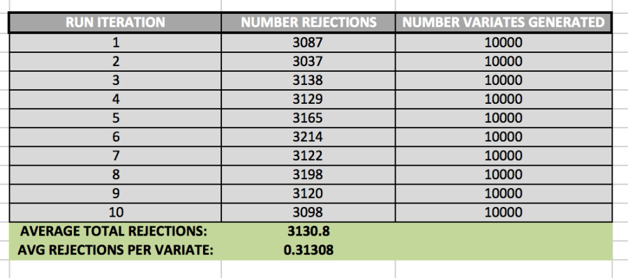
It is also important to keep track of how many rejections we get while using the Accept/Reject method. In order to determine the average number of rejections, I ran the algorithm 10 times. The data set it created is shown below:
While generating 10,000 variates, the algorithm created 3130.8 rejections, on average. This means that, generally, there was about 1 rejected variate for every 3 valid variates.
Polar-Coordinate Method
In the Polar-Coordinate method, we take advantage of trigonometric properties by generating random variables uniformly distributed over (0, 2pi), and then transforming them into rectangular coordinates. This method, called the Box-Muller Method more formally, is not computationally efficient, however, because it involves use of logs, sines, and cosines—all expensive operations on a CPU.
In order to perform this operation more efficiently, I’ve used the method outlined by Sheldon Ross, on page 83 of his book Simulation (5th Ed.).
Step 1: Generate random numbers, U1 and U2
Step 2: Set V1 = 2U1 – 1, V2 = 2U2 – 1, S = V12 + V22
Step 3: If S > 1, return to Step 1.
Step 4: Return the independent standard normal for two variables, X and Y:
Where:
X = sqrt(-2*log(S)/2) * V1,
Y = sqrt(-2*log(S)/S)*V2
Expectations
Prior to running the experiment, I expected the Inverse-Transform Method to generate the worst variables themselves, because it only uses an approximation of the Standard Normal CDF, not the CDF itself. I was a little nervous about using an approximation for a CDF with no closed form to generate my inverse function, thinking that while our inverse may deliver results that are more or less reasonable, the resulting data set wouldn’t pass more advanced statistical tests since we are presumably losing precision, through the approximation process. But that said, I also expected its time efficiency to be the best, because we are only calculating logarithm each time we call the inverse function, and this seems to be the only slow operation.
I expected that method 2, Accept/Reject generate the most accurate variables, mostly because of the convincing mathematical proofs describing its validity on pages 77 and 78 of Ross’s Simulation textbook. Intuitively, the proof for this method makes sense, so I expected its data set to look most like something that truly follows the Standard Normal Distribution. From a time efficiency standpoint however, I expected this algorithm to perform 2nd best, because I’m using a logarithm each time I generate an exponential random variable. And with 2 log calls for each run, it seems like this method would be relatively slow, under the assumption that Python’s log function is expensive. (Log calls are used here because we know that –logU is exponential with rate lambda=1. But we need exponential variables generated with rate 1 for each Y variable, Y1 and Y2.)
The Polar Coordinate Method is the most abstract for me, and so I had a hard time seeing exactly why it would generate Standard Normal Random variables, and because of this, I wasn’t sure what to expect of its data set. I took it on faith that it would generate the correct variables, but I didn’t fully understand why. Moreover, I also expected it to perform the worst from a runtime perspective because it involves the most expensive operations: Two Square Roots and Two Log calls for each successful run.
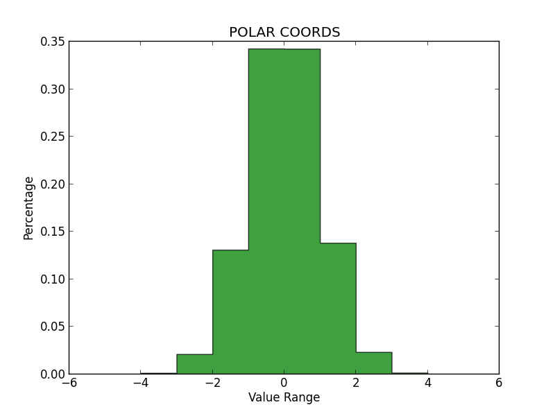
Histograms and Analysis
In order to determine whether each method produced qualitatively accurate data, I then plotted histograms for the numbers generated by each. All three histograms can be seen below. On my examination, it appears that the Inverse Transform yielded the least accurate representation, while the Polar Coordinate Method and Accept/Reject were much better, and about equal in validity.
Notably, the Inverse Transform method generated many values beyond the expected range of the Standard Normal (greater than 4.0 and less than -4.0). And while these values are possible, it seems like too many outliers—more than we would see in a true Standard Normal Distribution. Again, I think this is because we are using an approximation for the CDF, rather than the true Inverse of the CDF itself. I had some trouble getting these graphs to sit in-line, so please review the appendix to see them.
Chi-Squared Test
In order to determine wither the numbers generated may be from the Normal Distribution, I ran each method 10 times, and performed a Chi-Square test on each result. The data set can be seen in the tables within the appendix at the back of this document.
From this test, I was able to make the following determinations:
Inverse Transform:
N=10,000
Avg Chi Sq: 2,806.719
From 10 tests, each n=10,000
Critical Value:749
Result: REJECT Null Hypothesis
Accept/Reject
N=10,000
Avg Chi Sq: 10,025.226
From 10 tests, each n=10,000
Critical Value: 10,233.749
Result: ACCEPT Null Hypothesis
Accept/Reject
N=10,000
Avg Chi Sq: 9,963.320
From 10 tests, each n=10,000
Critical Value: 10,233.749
Result: ACCEPT Null Hypothesis
Runtime Analysis
Again, I ran each method 10 times to collect a sample of data with which to analyze runtime.
The average runtimes from 10 tests with n=10,000 were:
Inverse Transform: -6.60E-06 seconds
Accept/Reject: -5.72E-06 seconds
Polar Coordinates: –63E-06 seconds
This result was indeed surprising. I had expected the Polar Coordinates method to perform the worst, and it did—but only by a very small margin. Moreover, I had expected Inverse Transform to perform the best, and it was only fractions of a microsecond (or nanosecond?) faster than Polar Coordinates on average. I did not expected Accept/Reject to perform so well, but it was by far the fastest overall.
Conclusion
Given these results, I would recommend the Accept/Reject method for anyone who needs to generate Standard Normal Random Variables in Python (at least using my same implementations).
Accept/Reject not only passed the Chi-Square test at the 95% significance level, it also was by far the fastest of the three algorithms. It is roughly comparable to Polar Coordinates on the quality of variables generated, and it beats everything else on speed.
This file contains hidden or bidirectional Unicode text that may be interpreted or compiled differently than what appears below. To review, open the file in an editor that reveals hidden Unicode characters. Learn more about bidirectional Unicode characters
I generated some random numbers with a few different generators, some of which I made, and also used the one provided directly by Python. I wanted to see what the best option is for generating random numbers in a few simulations I’m doing.
It’s commented and can be run by simply invoking Python with: “python lcg.py”
I tried to explain what I was doing at each step to make this clear even for the comparatively un-initiated to the more esoteric statistics at play here, which aren’t totally necessary to know, and really will just be an impediment to __getting_started_now__. I wanted to share something so that people who are practically-minded like me can just jump in, start messing around, and know what to expect. So hopefully with just this code (full repo linked below) and the information presented here, you can start messing around with random number generators if you need to for any reason. (Most common reason would be to seed random variates in a simulation.)
My main goal in posting this is to give anyone with an interest in generating randomness an easy entry into it–with working code for these sort of generators, as it’s somewhat hard to find online, and the details can be a bit opaque, without clear examples of what to expect when you’re testing. So ideally, this will be the total package. Probably not, but hey, giving it a try. If for some reason you need help, feel free to contact me.
Random Number Generation
Generating truly random numbers is a longstanding problem in math, statistics, and computer science. True randomness requires true entropy, and in many applications—such as generating very large sets of random numbers very quickly—sufficient “true” entropy is difficult or impractical to obtain. (Often, it needs to come from the physical environment, sources such as radioactive decay, etc.) So, instead, we look to algorithmic random numbergenerators for help.
Algorithmically generated random numbers will never be “truly” random precisely because they are generated with a repeatable algorithmic formula. But for purposes such as simulating random events – these “Pseudo-random” numbers can be sufficient. These algorithmic generators take a “seed value” from the environment, or from a user, and use this seed as a variable in their formula to generate as many random-like numbers as a user would like.
Naturally, some of these algorithms are better than others, and hundreds (if not thousands, or more) of them have been designed over the years. The output is always deterministic, and never “truly” random, but the ideal goal is to approximate randomness by generating numbers which:
Are uniformly distributed on the range of [0,1)
Are statistically independent of each other
(That is, the outcomes of any given sequence do not rely on previously generated numbers)
The best random number generators will pass statistical tests for both uniformity and independence. In this analysis, we will subject three different random number generation algorithms to series of statistical tests and compare the outcomes.
The algorithms we will test are:
Python’s Built-In Random Number Generator
This algorithm is called the “Mersenne Twister”, implementation details are available at: Python Docs for Random
Seed value: 123456789
A Linear Congruential Generator
Seed value: 123456789
a=101427
c=21
m=216
A Linear Congruential Generator with RANDU initial settings
Seed value: 123456789
a=65539
c=0
m=231
The tests each algorithm will be subjected to are:
Uniformity tests
Chi-squared Test for Uniformity
Kolmogorov-Smirnov Test for Uniformity
Null hypothesis for BOTH tests: The numbers in our data set are uniformly distributed
Independence tests
Runs Test for Independence
Autocorrelation Test for Independence, (gap sizes: 2,3,5, and 5 will be used)
Null hypothesis for BOTH tests: The numbers in our data set are independent of each other
Test Result Summary & Quick Notes on Implementation
The exact implementation of each test can be viewed in the linked Python file named: “lcg.py”. The tests can be duplicated by anyone with Python installed on their system by running the command “python lcg.py”.
You can view the file directly on GitHub here: >> lcg.py <<
SUMMARY TABLE (2.1)
Algorithm
X2
TS/Result
KS TS/Result
Runs
TS/ Result
Autocorrelation
TS/Result
Mersenne Twister (PyRand)
9.754
Pass all
0.079213
Pass all
-1.6605
Reject at 0.8 and 0.9
Pass at 0.95
Gap=2: -1.089
Gap=3: -0.924
Gap=5: -0.559
Gap=50: -0.228
All Pass
LGC
6.288
Pass all
0.0537888
Pass all
0.5218
Pass all
Gap=2: 0.1753
Gap=3: -0.394
Gap=5: 0.872
Gap=50: 1.335
Reject at 0.8, Gap=50, others pass
LGC, w/ RANDU
12.336
Pass all
0.053579
Pass all
-0.2135
Pass all
Gap=2: -0.6591
Gap=3: -0.9311
Gap=5: 0.5788
Gap=50:-0.9093
All pass
The summary table above shows each algorithm tested, and which tests were passed or failed. More detailed output for each test and for each algorithm can be viewed in Tables 1.1 – 1.3 in the appendix to this document.
The Kolmogorov-Smirnov (or KS test) was run at the following levels of significance: .90, 0.95, 0.99. The formulas for the critical value at these significance levels were taken from table of A7 of Discrete-Event System Simulation by Jerry Banks and John S. Carson II. (Formulas for 0.80 could not be found, so I’ve used what was available.)
All other tests were run at the 0.80, 0.90., and 0.95 significance level.
Statistical Analysis and Expectations
Prior to generating the numbers for each test, I expected Python’s random function to perform the best of all three algorithms tested, mostly because it’s the library random function of one of the world’s most popular programming languages. (Which means: thousands and thousands of code repositories rely on it—many of which are used by commercial and mission critical programs.) But in fact, it performed the worst, failing the Runs Test at both the 0.80 and 0.90 level of significance. These failings are NOT statistically significant at the alpha=0.05 level, but it’s still surprising to see.
I expected the RANDU algorithm to perform the worst, and I thought it would perform especially badly on the autocorrelation test. This is because RANDU is known to have problems, outlined here. Specifically, it is known to produce values which fall along only a specific set of parallel planes (visualization in link above), which means the numbers should NOT be independent, when tested at the right gap lengths. It’s possible that the gap lengths I’ve tested simply missed any of these planes, and as a result—RANDU performed the best of all the algorithms. It’s the only algorithm that didn’t fail any statistical tests at all.
I anticipated the LGC function to perform 2nd best overall, and I was right about that—but the best and worst algorithm were the opposite of what I expected. Mostly, I thought that that Python’s random generator would be nearly perfect, RANDU would be badly flawed, and the LGC would be just okay. Really, the LGC performed admirably: The only test it failed was autocorrelation at the 0.80 confidence level, and that isn’t statistically significant by most measures.
Reviewing the data output into each .txt file directly, I don’t see any discernible patterns in the numbers themselves. And with 10,000 data points, there’s so much output to review that I can see why statistical measures are needed to effectively to determine what’s really going on in the data. It’s probably possible to find a few patterns, specifically related to runs and gap-sequences just by viewing the data directly, but tests are still needed to find out for sure.
With that said, I do think the testing done in this experiment is sufficient, because we have two tests for each measure that matters: 1) Uniformity; 2) Independence. The only improvement I would make for future tests is testing more gap-sequences, and starting them at different points. I’d do this mostly because I know that RANDU should fail gap-sequence tests given the right input, but there would be some trial and error involved in trying to find these sequences naively. So, sometimes, getting into math itself and working with proofs may still be the most effective method. Maybe sometime the old-fashioned way is still best.
TABLE 1.2 – Linear Congruential Generator (X0 = 123456789 )
Test Name
Sample Size
Confidence Level
Critical Value
Test Statistic Found
Result
Chi-Square
10,000
0.80
10118.8246
6.288
FAIL TO REJECT null
Chi-Square
10,000
0.90
10181.6616
6.288
FAIL TO REJECT null
Chi-Square
10,000
0.95
10233.7489
6.288
FAIL TO REJECT null
Kolmogorov-Smirnov
100
0.90
0.122
0.05378
FAIL TO REJECT null
Kolmogorov-Smirnov
100
0.95
0.136
0.05378
FAIL TO REJECT null
Kolmogorov-Smirnov
100
0.99
0.163
0.05378
FAIL TO REJECT null
Runs Test
10,000
0.80
1.282
0.521889
FAIL TO REJECT null
Runs Test
10,000
0.90
1.645
0.521889
FAIL TO REJECT null
Runs Test
10,000
0.95
1.96
0.521889
FAIL TO REJECT null
Autocorrelation,
GapSize=2
10,000
0.80
1.282
0.175377
FAIL TO REJECT null
Autocorrelation,
GapSize=2
10,000
0.90
1.645
0.1753777
FAIL TO REJECT null
Autocorrelation,
GapSize=2
10,000
0.95
1.96
0.1753777
FAIL TO REJECT null
Autocorrelation,
GapSize=3
10,000
0.8
1.282
-0.39487
FAIL TO REJECT null
Autocorrelation,
GapSize=3
10,000
0.9
1.645
-0.39487
FAIL TO REJECT null
Autocorrelation,
GapSize=3
10,000
0.95
1.96
-0.39487
FAIL TO REJECT null
Autocorrelation,
GapSize=5
10,000
0.8
1.282
0.872668
FAIL TO REJECT null
Autocorrelation,
GapSize=5
10,000
0.9
1.645
0.872668
FAIL TO REJECT null
Autocorrelation,
GapSize=5
10,000
0.95
1.96
0.872668
FAIL TO REJECT
null
Autocorrelation,
GapSize=50
10,000
0.8
1.282
1.3352
REJECT null
Autocorrelation,
GapSize=50
10,000
0.9
1.645
1.3352
FAIL TO REJECT null
Autocorrelation,
GapSize=50
10,000
0.95
1.96
1.3352
FAIL TO REJECT null
Test Name
Sample Size
Confidence Level
Critical Value
Test Statistic Found
Result
END TABLE 1.2
TABLE 1.3 – Linear Congruential Generator with RANDU initial settings


You must be logged in to post a comment.