Note: I am experimenting with exporting Jupyter notebooks into a WordPress ready format. This notebook refers specifically to to the Nature Conservancy Kaggle, for classifying fish species, based only on photographs.
For awhile now, the Computer Science department at my University has offered a class for non-CS students called “Data Witchcraft“. The idea, I suppose, is that when you don’t understand how a technology works, it’s essentially “magic“. (And when it has to do with computers and data, it’s dark magic at that.)
But even as someone who writes programs all day long, there are often tools, algorithms, or ideas we use that we don’t really understand–just take at face value, because well, they seem to work, we’re busy, and learning doesn’t seem necessary when the problem is already sufficiently solved.
One of the more prevalent algorithms of this sort is Gradient Descent (GD). The algorithm is bothconceptually simple (everyone likes to show rudimentary sketches of a blindfolded stick figure walking down a mountain) and mathematically rigorous (next to those simple sketches, we show equations with partial derivatives across n-dimensional vectors mapped to an arbitrarily sized higher-dimensional space).
So most often, after learning about GD, you are sent off into the wild to use it, without ever having programmed it from scratch. From this view, Gradient Descent is a sort of incantation we Supreme Hacker Mage Lords can use to solve complex optimization problems whenever our data is in the right format, and we want a quick fix. (Kind of like Neural Networks and “Deep Learning”…) This is practical for most people who just need to get things done. But it’s also unsatisfying for others (myself included).
However, GD can also be implemented in just a few lines of code (even though it won’t be as highly optimized as an industrial-strength version).
That’s why I’m sharing some implementations of both Univariate and generalized Multivariate Gradient Descent written in simple and annotated Python.
Anyone curious about a working implementation (and with some test data in hand) can try this out to experiment. The code snippets below have print statements built in so you can see how your model changes every iteration.
But the actual algorithms are also extracted below, for ease of reading.
Univariate Gradient Descent
Requires NumPy.
Also Requires data to be in this this format: [(x1,y1), (x2,y2) … (xn,yn)], where Y is the actual value.
This file contains hidden or bidirectional Unicode text that may be interpreted or compiled differently than what appears below. To review, open the file in an editor that reveals hidden Unicode characters. Learn more about bidirectional Unicode characters
Also Requires data to be in this this format: [(x1,..xn, y),(x1,..xn, y) …(x1,..xn, y)], where Y is the actual value. Essentially, you can have as many x-variables as you’d like, as long as the y-value is the last element of each tuple.
This file contains hidden or bidirectional Unicode text that may be interpreted or compiled differently than what appears below. To review, open the file in an editor that reveals hidden Unicode characters. Learn more about bidirectional Unicode characters
In which I peel back the curtain and outline the innerworkings of a particularly insidious artificial intelligence, whose sole purpose in life is to systematically learn the optimal strategy for a terrifyingly addictive video game, known only to the internet as: Flappy Bird… and in which I also provide code to program a similar AI of your own.
More pointedly, this short post outlines a practical way to get started using a Reinforcement Learning technique called Q-Learning, as applied to a PythonFlappy Bird clone, programmed by @TimoWilken.
So you want to beat Flappy Bird, but after awhile it gets tedious. I agree. Instead, why don’t we program an AI to do it for us? A genius plan, but where do we start?
First, we need a Flappy Bird game to hack upate. The candidate that I suggest is a Python implementation created by Timo Wilken and available for download directly at: https://github.com/TimoWilken/flappy-bird-pygame. This Flappy Bird version is implemented using the PyGame library, which is a dependency going forward.
The first challenge we’ll have in implementing the framework for a Flappy AI is determining exactly how the game workes in its original state.
By using the debugger and stepping through the game’s code during some trial runs, I was able to figure out where key decisions where made, how data flowed into the game, and exactly where I would need to position my AI-agent.
At its basic level, I created an “Agent” class, and passed that class into the running game code. Then, at each loop of the game, I examined the variables available to me, and then passed a ‘MOUSEBUTTONUP’ command to the PyGame event queue whenever the AI decided to jump. Otherwise, I did nothing.
State Representations
From there, the next step was determining a way to model the problem. I decided to use follow the basic guidelines outlined by Sarvagya Vaish, here.
First, I discretized the space in which the bird sat, relative to the next pipe. I was able to get pipe data by accessing the pipe object in the original game code. Similarly, I was able to get bird data by accessing the bird object.
From there, I could determine the location of the bird and the pipesrelative to each other. I discretized this space as a 25×25 grid, with the following parameters:
This file contains hidden or bidirectional Unicode text that may be interpreted or compiled differently than what appears below. To review, open the file in an editor that reveals hidden Unicode characters. Learn more about bidirectional Unicode characters
Then, each iteration of the game loop, I was able to determine the bird’s relative position, and whether it had made a collision with the pipes or not.
If there was no collision, I issued a reward of +1.
If there was a collision, I issued a reward of -1000.
I tried many different state representations here, but mostly it was matter of determining an optimal number of grid spaces and the right parameters for those spaces.
Initially, I started with a 9×9 grid, but moved to 16×16 because I got to a point in 9×9 where I just couldn’t make any more learning progress.
What Works
Very generally, we want to have a tighter grid around the pipes, as this is where most collisions happen. And we want a looser grid as we move outwards. This seemed to give me the best results, as we need different strategies at different locations on the grid.
Exploration Approaches
Our next task is implementing an exploration approach. This is necessary because if we don’t randomly explore the state sometimes, there might be optimal strategies that we are never able to find, simply because we will never be in those states!
Because we have only two choices at any given state (JUMP—or—STAY), implementing exploration was relatively simple.
I started out with a high exploration factor (I used 1/time_value+1), and then I generated a random number between [0,1). If the random number was less than the exploration factor, then I explored.
Over time the exploration factor got lower, and therefore the AI explored less frequently.
Exploration essentially consisted of flipping a fair coin (generating a Boolean value randomly).
If true: then I chose to JUMP.
If false: I chose to STAY.
The main problem I encountered with this method is that the exploration factor was very at the beginning, and sometimes choices were made that were not representative of actual situations that the bird would encounter in ‘true’ gameplay.
BUT, because these decisions were made earlier, they were weighted more heavily in the overall Q-Learning algorithm.
This isn’t ideal, but exploration is necessary, and overall the algorithm works well. So it wasn’t a large problem, overall.
Learning Rates & Their Impact
Very simply, “Learning Rates” dicatate how much we weigh new information about some state over old information. Learning rates can be an value in the range [0,1]. With 0 meaning we never update values (bad), and 1 meaning that we only EVER care about what happened the last time we were in state (short-sighted).
The first learning rate I tried was alpha=(1/time+1). However, this gave very poor results in practice.
This is because time is NOT the most important factor in determining a strategy from any given state. Rather, it is how many times we’ve been to that state.
The problem is that we make extremely poor choices at the beginning of the game (because we simply don’t know any better). But with alpha=(1/time+1), the results of these these poor choices are weighted the most highly.
Once I changed the learning factor to alpha=1/N(s,a), I immediately saw dramatically better results. (That is, where N(s,a) tracks how many times we’ve been in a given state and performed the same action.)
Training
My final, “Smart” bird is the result of about 4 hours of training.
I don’t actually think there would be a way to make the training more efficient, aside from speeding up the gameplay in some way.
Overall, I the results I received from the investment of time I put it in reasonable.
Given more time, I would probably discretize the space even more finely (maybe a 36×36 grid) – so that I could find even more optimal strategies from a more fine-tuned set of positions in the game-space.
How to Use my Smart Bird
To use my smart bird, simply take the following steps:
cd into a directory containing my source code
Ensure that this directory includes the file named ‘txt’
Run the command:
python flappybird.py “qdata.txt”
Watch Flappy crush it. (the game will run 10x)
Learning From Scratch
Probably more instructive than using my trained bird though, is to simply start training a new bird from scratch. You will see the agony and the ecstasy as he does a terrible number of dumb things, slowly learning how to beat the game.
It’s surprisingly enjoyable (though sometimes frustrating) and highly recommended. Start the process by running:
python flappybird.py
With no other args. Then pass in the ‘qdata.txt’ file next time you run the game, to keep your learning session going.
Citations
I consulted the following resources to implement my AI. If you want to do similar work, I’d recommend these resources. These people are much smarter than me. I’m just applying their concepts.
While studying Operating Systems, I decided to experiment with 4 of the most common Page Replacement algorithms, via simulation, using Python. Input data for my simulations were two memory traces named “swim.trace” and “gcc.trace” (provided by my CS department). All algorithms are run within a page table implemented for a 32-bit address space; all pages in this page table are 4kb in size.
I chose to implement these algorithms and the page table in Python. The final source code can be found here, on Github. The full data set that I collected can be found at the end of this document. Illustrative graphs are interspersed throughout, wherever they are necessary for explaining and documenting decisions.
In this essay itself, I will first outline the algorithms implemented, noting design decisions I made during my implementations. I will then compare and contrast the results of each algorithm when run on the two provided memory traces. Finally, I will conclude with my decision about which algorithm would be best to run in a real Operating System.
Please note, to run the algorithms themselves, you must run:
python vmsim.py –n -a <opt|clock|aging|lru> [-r ]
The Algorithms
The algorithms we have been asked to implement are:
Opt– Simulate what the optimal page replacement algorithm would choose if it had perfect knowledge
EXAMPLE RUN: python vmsim.py –n 8 –a opt gcc.trace
Clock– Use the better implementation of the second-chance algorithm
EXAMPLE RUN: python vmsim.py –n 16 –a clock swim.trace
Aging– Implement the aging algorithm that approximates LRU with an 8-bit counter
EXAMPLE RUN: python vmsim.py –n 64 –a lru swim.trace
Implementation Notes
The main entry point for the program is the file named vmsim.py. This is the file which must be invoked from the command line to run the algorithms. Because this is a python file, it must be called with “python vmsim.py … etc.”, instead of “./vmsim”, as a C program would. Please make sure the selected trace file is in the same directory as vmsim.py.
All algorithms run within a page table, the implementation of which can be found in the file named pageTable.py.
Upon program start, the trace file is parsed by the class in the file parseInput.py, and each memory lookup is stored in a list of tuples, in this format: [(MEM_ADDRESS_00, R/W), [(MEM_ADDRESS_01, R/W), … [(MEM_ADDRESS_N, R/W)]. This list is then passed to whichever algorithm is invoked, so it can run the chosen algorithm on the items in the list, element by element.
The OPT algorithm can be found in the file opt.py. My implementation of OPT works by first preprocessing all of the memory addresses in our Trace, and creating a HashTable where the key is our VPN, and the value is a python listcontaining each of the address numbers at which those VPNs are loaded. Each time a VPN is loaded, the element at index 0 in that list is discarded. This way, we only have to iterate through the full trace once, and from there on out we just need to hash into a list and take the next element, whenever we want to know how far into the future that VPN is next used.
The Clock Algorithm is implemented in the files clock.py and circularQueue.py. My implementation uses the second chance algorithm with a Circular Queue. Of importance: whenever we need to make an eviction, but fail to find ANY pages that are clean, we then run a ‘swap daemon’ which writes out ALL dirty pages to disk at that time. This helps me get fewer page faults, at the expense of more disk writes. That’s a calculated decision for this particular algorithm, since the project description says we should use page faults as our judgment criterion for each algorithm’s effectiveness.
The LRU Algorithm can be found in the file lru.py. For LRU, each time a page is Read, I mark the memory address number at which this happens in the frame itself. Then, in the future—whenever I need to make an eviction—I have easy access to see which frame was used the longest time in the past, and no difficult calculations are needed. This was the simplest algorithm to implement.
The Aging Algorithm is likely the most complex, and its source code can be found in the file named aging.py. Aging works by keeping an 8 bit counter and marking whether each page in the page table was used during the last ‘tick’ a time period of evaluation which must be passed in by the user as a ‘refresh rate’, whenever the Aging Algorithm is selected. All refresh rates are in milliseconds on my system, but this relies on the implementation of Python’s “time” module, so it’s possible that this could vary on other systems. For aging, I suggest a refresh rate of 0.01 milliseconds, passed in on the command line as “-r 0.01”, in the 2nd to last position in the arg list. This minimizes the values in my testing, and going lower does not positively affect anything. In the next section, I will show my rationale for selecting 0.01 as my refresh rate.
Aging Algorithm Refresh Rate
In order to find a refresh rate that would work well, I decided to start at 1ms and move 5 orders of magnitude in each direction, from 0.00001ms to 100000ms.
To ensure that the results were not biased toward being optimized for a single trace, I tried both to confirm that the refresh rate would work will for all inputs.
The graphs below show the Page Faults and Disk Writes I found during each test.
For all tests, I chose a frame size of 8, since this small frame size is most sensitive to the algorithm used.At higher frame sizes, all of the algorithms tend to perform better, across the board. So I wanted to focus on testing at the smallest possible size, preparing for a ‘worst case’ scenario.
Aging Algorithm – Page Faults Over Refresh Rate
X-axis: Refresh rate in milliseconds
Y-axis: Total Page faults
GCC. TRACE reaches its minimum for page faults at 0.0001ms and SWIM.TRACE reaches its own minimum at 0.01ms. The lines cross at around 0.01ms.
Total Page Faults For SWIM.TRACE – Detail
X-axis: Page Faults
Y-Axis: Refresh Rates
X-axis: Page Faults
Y-Axis: Refresh Rates
Additionally, 0.01ms seems to achieve the best balance, in my opinion, if we need to select a single time for BOTH algorithms.
Aging Algorithm – Disk Writes Over Refresh Rate
X-axis: Refresh rate in milliseconds
Y-axis: Total Disk Writes
The number of disk writes also bottoms out at 0.01ms from SWIM.TRACE. It is relatively constant for GCC.TRACE across all of the different timing options.
Because of this, I suggest 0.01ms as the ideal refresh rate. This is because it is optimal for SWIM.TRACE. For GCC.TRACE, it is not the absolute best option, but it is still acceptable, and so I think this selection will achieve a good balance.
Results & Decisions
With the algorithms all implemented, my next step was to collect data for each algorithm at all frame sizes, 8, 16, 32, and 64. OPT always performed best, and thus it was used as our baseline.
In the graphs below, I show how each algorithm performed, both in terms of total page faults and total disk writes.
SWIM.TRACE – Page Faults Over Frame Size
X-axis: Frame Size
Y-axis: Page Faults
Data for all algorithms processing swim.trace
SWIM.TRACE – Disk Writes Over Frame Size
X-axis: Frame Size
Y-axis: Disk Writes
Data for all algorithms processing swim.trace
GCC.TRACE – Page Faults Over Frame Size
X-axis: Frame Size
Y-axis: Page Faults
Data for all algorithms processing gcc.trace
GCC.TRACE – Disk Writes Over Frame Size
X-axis: Frame Size
Y-axis: Disk Writes
Data for all algorithms processing gcc.trace
—
Given this data, I was next tasked with choosing which algorithm is most appropriate for an actual operating system.
In order to determine which algorithm would be best, I decided to use an algorithm. I’ll call it the ‘Decision Matrix’, and here are the steps.
DECISION MATRIX:
RANK ALGORITHMS FOR EACH CATEGORY FROM 1=BEST to 4=WORST,
SELECT ALGORITHM WITH LOWEST OVERALL SCORE
ALGORITHM
SWIM – Page Faults
SWIM – Disk Writes
GCC – Page Faults
GCC – Disk Writes
TOTAL (Lowest is Best)
OPT
1
1
1
1
4
CLOCK
2
4
2
4
12
AGING
4
2
4
2
12
LRU
3
3
3
3
12
Ranking: 1=Best;
4=Worst
NOTE:
Wherever lines cross each other in our graphs, the algorithm ranked as “better” is the one with MORE total low data points. Ties were broken by my own personal judgment.
Decision:
Of course, using this set of judgment criteria, OPT is by far the winner.
However OPT isn’t an option in a real OS, since it requires perfect knowledge of the future, which is impossible in practice.
So we want to pick between the 3-way tie for CLOCK and LRU and AGING.
Of these three:
AGING does well on disk writes, but generally has the most page faults.
Conversely, CLOCK does well on page faults, but often has the most disk writes.
LRU achieves a balance.
Therefore, My pick goes to LRU, because where clock does beat LRU, on page faults it does so only by a narrow margin.
But where LRU beats clock—on disk writes—it does so by a large amount. This means LRU is better overall, if both page faults and disk writes are equally weighted for judgment purposes.
Therefore, I would select LRU for my own operating system.
Teleology (a.k.a – what is the purpose of this post?)
Recently, I finished an artificial intelligence project that involved implementing the Minimax and Alpha-Beta pruning algorithms in Python.
These algorithms are standard and useful ways to optimize decision making for an AI-agent, and they are fairly straightforward to implement.
I haven’t seen any actual working implementations of these using Python yet, however. So I’m posting my code as an example for future programmers to improve & expand upon.
It’s also useful to see a working implementation of abstract algorithms sometimes, when you’re seeking greater intuition about how they work in practice.
My hope is that this post provides you with some of that intuition, should you need it–and that it does so at an accelerated pace.
Ontology (a.k.a – how does this abstract idea __actually work__, in reality?)
Let’s start with Minimax itself.
Assumptions: This code assumes you have already built a game tree relevant to your problem, and now your task is to parse it. If you haven’t yet built a game tree, that will be the first step in this process. I have a previous post about how I did it for my own problem, and you can use that as a starting point. But keep in mind that YMMV.
My implementation looks like this:
This file contains hidden or bidirectional Unicode text that may be interpreted or compiled differently than what appears below. To review, open the file in an editor that reveals hidden Unicode characters. Learn more about bidirectional Unicode characters
How-to: To use this code, create a new instance of the Minimax object, and pass in your GameTree object. This code should work on any GameTree object that has fields for: 1) child nodes; 2) value. (That is, unless I made an error, which of course, is very possible)
After the Minimax object is instantiated, run the minimax() function, and you will see a trace of the program’s output, as the algorithm evaluates each node in turn, before choosing the best possible option.
What you’ll notice: Minimax needs to evaluate **every single node** in your tree. For a small tree, that’s okay. But for a huge AI problem with millions of possible states to evaluate (think: Chess, Go, etc.), this isn’t practical.
How we solve: To solve the problem of looking at every single node, we can implement a pruning improvement to Minimax, called Alpha-Beta.
Alpha-Beta Pruning Improvement
Essentially, Alpha-Beta pruning works keeping track of the best/worst values seen as the algorithm traverses the tree.
Then, if ever we get to a node with a child who has a higher/lower value which would disqualify it as an option–we just skip ahead.
Rather than going into a theoretical discussion of WHY Alpha-Beta works, this post is focused on the HOW. For me, it’s easier to see the how and work backwards to why. So here’s the quick and dirty implementation.
This file contains hidden or bidirectional Unicode text that may be interpreted or compiled differently than what appears below. To review, open the file in an editor that reveals hidden Unicode characters. Learn more about bidirectional Unicode characters
How-to: This algorithm works the same as Minimax. Instantiate a new object with your GameTree as an argument, and then call alpha_beta_search().
What you’ll notice: Alpha-Beta pruning will alwaysgive us the same result as Minimax (if called on the same input), but it will require evaluating far fewer nodes. Tracing through the code will illustrate why.
Phenomenology (a.k.a – how will I perceive this, myself?)
This isn’t the most robust implementation of either algorithm (in fact it’s deficient in many ways), so I wouldn’t recommend it for industrial use.
However, this code should simply illustrate how each algorithm works, and it will provide output you can trace through and compare against–as long as you are able to construct the GameTree for your problem.
From there, it’s only a matter of time until you’ll understand it intuitively. This is one of those things that took a little while for me to grasp–so hopefully having a clear example will help others get there more quickly. Good luck.
I need to parse and build tree which has an arbitrary branching factor, and values only at the leaves.
(As for why: Later, I’ll be running Minimax and some other algorithms on this tree, in order to algorithmically determine the best possible game move. More on that in another post.)
This seemed like a good problem to solve recursively. And to avoid a soul-sucking debug session, I decided my goal was to solve it as succinctly as possible.
Here’s what I came up with. Why I’m posting: This seems like it would be a very common AI/Data-Structures problem, but my first few searches on the subject came up with nada. Nothing even closely related to the problem I’m solving. So doing my part to fix that now.
Working Code
This file contains hidden or bidirectional Unicode text that may be interpreted or compiled differently than what appears below. To review, open the file in an editor that reveals hidden Unicode characters. Learn more about bidirectional Unicode characters
Side note. I’m actually not sure what this tree (with weights only at the leaves) would be called technically. It reminds me of the tree made during Huffman Encoding, but it’s not quite a match for that since we aren’t summing the values in all parent nodes. If you know the technical name, let me know, so I can update.
Example code to start experimenting with the Harris Corner Detection Algorithm on your own, in Matlab. And some of the results I obtained in my own testing.
Corner Cases
Among the classic algorithms in Computer Vision is Harris Corner Detection. (For the original paper, from 1988, see here.) The problem it solves: Given any image file, can you find which areas correspond to a corner with a high degree of certainty?
The answer is yes. And the algorithm is elegant. Essentially the steps are:
Convert your image to a Matrix, storing the pixel values by intensity (converting to B/W makes this easier)
Find the horizontal and vertical gradients of the image (essentially the derivative of pixel intensities). This will let us know where there are horizontal and vertical edges.
Scan the image getting groups of pixels for however wide an area you are concerned with, and perform a calculation to determine where the horizontal and vertical edges intersect. (This requires some relatively complex linear algebra, but I’m not focusing on the theory here, just the implementation.)
Recently, I was trying to implement my own version of the Harris Detector in Matlab, and ended up banging my head against the wall for a few hours while figuring out some of the subtler details the hard way.
Here’s the code I came up with, and some examples of the outputs. Grab the code from both gists below, and you can start experimenting on your own.
Harris Algorithm
This file contains hidden or bidirectional Unicode text that may be interpreted or compiled differently than what appears below. To review, open the file in an editor that reveals hidden Unicode characters. Learn more about bidirectional Unicode characters
This file contains hidden or bidirectional Unicode text that may be interpreted or compiled differently than what appears below. To review, open the file in an editor that reveals hidden Unicode characters. Learn more about bidirectional Unicode characters
Here’s what you can expect to see. I’m coloring the corners RED, using circles that grow larger the more likely the area is to hold a corner. So, larger circles –> more obvious corners. (Also note that I’m downsizing my output images slightly, just to make computation faster. )
Closing
That’s it. With this code, you can start experimenting with Harris Detectors in about 30 seconds. And hopefully the way I’ve written it is transparent enough to make it obvious what’s going on behind the scenes. Most of the implementations out there are somewhat opaque and hard to understand at a conceptual level. But I’m hoping that my contribution will make this all a little more straightforward to those just gettings started. Enjoy. -t
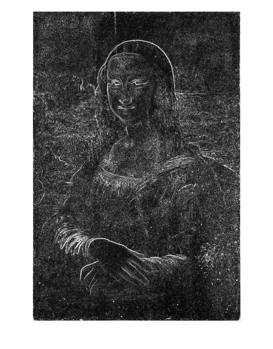
I’m currently working on a computer vision project to implement seam carving, which is explained quickly in this video by the technique’s inventors. The goal of seam carving is to allow for content-aware image resizing. Part of this algorithm is a numerical method to identify the ‘important’ content of an image (at least w/r/t re-sizing). I wanted to see what this algorithm would ID as ‘important’ in some great artworks from history. So I ran the algorithm on some of my favorite paintings (low-res versions from the internet) and am sharing the outputs here.
Brief Technical Explanation (skip if not interested)
The short story is that seam carving allows us to re-size images without distorting the important details. Seam carving is the process of finding connected paths of pixels with “low energy” running through the image–call these paths seams–and then removing those seams instead of a full column or row which might intersect with something important in the image, like a person’s face, the edge of a large object, etc… The easiest way to get an overview is to watch the video above, but hopefully that’s a succinct enough explanation for anyone impatient like me.
The first step in implementing the seam carving algorithm is to compute what’s called the energy function of the image’s pixel gradients. We can do this by plotting the image’s grayscale values (0-255) in a 2D matrix, applying a filter to identify edge gradients in both the x-direction and y-direction, and then computing the magnitude of each pixel’s edge gradient, weighing the x-gradient and y-gradient equally: (i.e. — sqrt(x^2 + y^2) ). If that doesn’t make a ton of sense yet, don’t worry. The video is the easiest way to understand the concept, and reading the paper is the easiest way to understand the process. This is just the super succinct version. (I also probably explained it badly.)
The Energy Function Code
This file contains hidden or bidirectional Unicode text that may be interpreted or compiled differently than what appears below. To review, open the file in an editor that reveals hidden Unicode characters. Learn more about bidirectional Unicode characters
Okay, so now we can compute the energy function of any image.
And the supposed output of this energy function is a mapping where the the important details of the image–the ones we don’t want to carve out when we re-size–are represented in higher intensities of white. The less important details of the image are represented in darker shades of gray and black.
So my question is what happens when we run historical artworks through this algorithm? Does it tell us anything new and novel about artist, his techniques, etc? I’ve always heard that the really well educated and expert art historians can confirm or deny the veracity of an artwork by looking at brush strokes, and the like. I’ve also read stories about taking x-rays of famous artworks, and revealing hidden paintings beneath.
For the most part I’ll let you decide, but in any case, I found some of the outputs to be really beautiful and interesting in their own right. Enough talking for now, here’s the imagery.
You’ll have to click through to see the images in full-size (bottom right button in popup after clicking on the thumbnail), and some of the more interesting details need magnification, which requires downloading the images, just as a heads up.
Da Vinci
Picasso
Bacon
El Greco
De Kooning
Vermeer
Closing
There’s a lot more that can be done with this, of course, and this post has no real analysis, conclusions, or anything of the like. But I wanted to share what I was playing around with, in case anyone else finds it interesting, like I do. -t
In which I suggest, quite longwindedly, that the next great avant-garde movement in art & music & writing will be AI-Assisted Creativity. I’ll probably edit this later, but it’s something I want to think through and am happy to talk with others about. I’m genuinely very interested in the future of art/creativity and also wondering about others’ opinions and views, where mine fall short, etc.
The First Realization of the Avant-Garde Dream
Before I got into software, I wanted to be an artist. My main focus was on avant-garde art, doing something new, and pushing boundaries—eventually with the goal of merging the mundanities of our everyday lives with our artistic output, such that the entirety of our existence becomes a single, continuous, expressive work of art.
This was the goal of the Happenings in the sixties, the Dadaists in the 20s, even Andy Warhol when he essentially suggested art was all around us, even at the grocery store. (In a strange way this is something akin to the old zen-philosophy, of fully *being* in every moment, seeing its beauty.) And it’s still the goal of performance art that breaks the boundaries between life and performance, like Sleep No More in NYC, and many others across the world. The point is this: you no longer know where reality ends and artifice begins. Because of this, ideally, everything is a form of joyful, creative expression, nothing is ‘work’, and we get lost in an ideal world where we can be artists not workers at some job we don’t care about.
At first, this seemed like a desirable goal to me, and it seemed like it was becoming increasingly possible with more and more online media outlets like YouTube, and Instagram, Facebook and others allowing us to document and color every moment of our lives however we’d like. Every meal, every night out, every workout, all of them can become part of the artwork that is your life—as you present it anyway—a sort of of online self portrait that’s always a work in progress and might just live forever as pure electricity flowing around our planet from satellite to satellite, computer to computer, long after you’ve turned to dust.
There’s something wild and Romantic about that notion, and back in 2009 or 2008, saying those kinds of things at art classes in a University got lots of people angry. But here we are, in 2016, and that’s more or less what happened at some level. Today, I’d suggest, the dream of the avant-garde of the 20th century has largely been fully realized: all of our lives are one continuous artwork, and every moment we’re making art, working on those self-portraits, whether we like it or not. We’re writing, we’re taking photos, films, always and obsessively critiquing.
However, the dream has been realized perversely. Rather than turn everything into joyful creativity, it’s turned all of our lives into one continuous exercise in content farming—it’s not artwork, it’s just **work**, and sometimes even __getting a job__ requires social media presence as a daily necessity. And more pointedly, rather than allowing using to create artwork for our own joy and benefit, we generally cede all copyrights to companies the second we hit post, send, or click.
None of this is news, but the point I’m intending to make is this: 1) In the 20th century, experimental artists desired to merge art and life together, this was called the avant-garde 2) By the early 21st century this dream has succeeded. In countries like the United States, many people spend their entire day creating artwork (writing, photos, videos) on platforms like Instagram, or YouTube, etc, Twitter, etc. 3) But rather than freeing artists from the strictures of work and labor, turning life into a wild, creative dream, it’s generally created a more subtle dystopia, where creating artwork is an extra necessary part of daily life 4) So, while the Avant-Garde dream has succeeded, it’s also failed, and in doing so, it’s planted the seeds for the next great trend in artistic innovation, namely: where do we go from here?
Where do we go from here?
Okay, so the Avant-garde dream succeeds, but it creates its own problems, at least in this conception. Now we’re all artists, but we’re giving away our artistic work & hence our very lives to companies that subtly control us in more ways than we really know, and we do so *by the very act* of creating the artwork that we’re more or less necessitated to produce in order to succeed in 21st century life. (When’s the last time you tried to apply for a job that didn’t want to see your personal ‘fun’ Github projects, your witty Twitter comments, or your LinkedIn profile?)
My suggestion is that the really innovative artists will take things one step further. They’ll attempt to merge our digital lives with the very algorithms that control them.
There’s long been a movement, in both software and art, to create programs that allow us to generate artwork, or music, or writing that is more or less indistinguishable from that created by a human. There are reasons for this, and besides being cool, it serves as a basis Turing Test of sorts for machine creativity and has implications for the P vs NP problem that forms the foundation of theoretical computer science. For instance: are all creative problems ‘solvable’ by computers in Polynomial time? And if so, aren’t we just computers, etc., etc…
That’s interesting stuff, but more interesting to me, and more groundbreaking is the idea of merging the computational infrastructure that makes up our digital lives with the artwork that we produce. That is: can we **use** AI algorithms to __supplement__ our creativity, rather than replace it altogether?
For example, here are two projects that I’ve come across recently which sparked my interest:
Both are attempts to computationally generate art that’s completely indistinguishable from human-created artwork. But they could be even better with a human touch. I think this kind of work is truly incredible, but only halfway there. We still need a human element, and by working with computers, we are taking the next step in avant-garde art, though I still wonder what the next set of repercussions may be.
Examples of what I’m thinking
Musical: A musical group where one of the improvising performers is an AI, and the others are reacting to this improvisation in real-time. This could be a way to spur creativity in the songwriting process.
Textual: Computationally generate a short story, or news article, and then have a human read through and improve it, cutting down the time to produce high-quality content by a huge factor
Visual: Computationally generate dozens of images based on some input criteria, maybe just the mood you’re in or ideas you have, then improve upon these for your final artwork
Practical Thoughts: Outsourcing Creative Work
The theme here is outsourcing creative work to computers, so *we* can produce higher quality work in shorter periods of time. Just like your programming IDE can generate the outline of your project, why not have an AI generate the outline of your novel?
Ideally, in doing so, we’ll be taking the next step in avant-garde art by once again rebelling against the idea of being forced to do ‘work’, outsourcing the hard/boring stuff to computers, and only making art that’s fun for us: when we feel like it, and how we feel like it. An algorithm can either subtly control us, or it can do our chores.


You must be logged in to post a comment.