tl;dr
I needed to generate Standard Normal Random Variates for a simulation I’m programming, and I wanted to see which method would be best to use. There are a few options, but generally you need to experiment to know for sure which will work best in your situation.
I decided to do this in Python, and to share my code + experimentation process and recommendations/reasoning.
Hoping this can save someone else some time later. If you need to do the same for your own simulation, or any other reason, hopefully this solves some of your problems, helps you understand what’s going on under the hood, and just makes life easier.
Grab the code here: https://github.com/adpoe/STD-Normal-Rand-Variates/tree/master/code
Generating Random Variates from Standard Normal
Experimental Setup
I used Python to algorithmically generate random variates that follow the Standard Normal distribution according to three different methods. For all methods, 10,000 valid random variables were generated in each algorithm’s run, in order to maintain consistency for later effectiveness comparisons. The methods tested were:
- The Inverse Transform Method
- The Accept/Reject Method
- The Polar-Coordinates Method
In the following paragraphs, I will briefly outline the implementation decisions made to generate Standard Normal random variates according to each method. I will then analyze the results, compare them, and issue my own recommendation on which method to use going forward, informed by the data gathered in this experiment.
Inverse Transform
The Inverse Transform Method works by finding the inverse of the CDF for a given probability distribution (F-1(X)), then feeding random numbers generated from U[0,1) into that inverse function. This will yield randomly generated variables within the range of our desired probability distribution.
However, this method is problematic for the Standard Normal Distribution, because there is no closed form for its CDF, and hence we cannot calculate its exact inverse. Because of this, I chose to use Bowling’s closed-form approximation of the Standard Normal CDF, which was developed in 2009: Pr(Z <= z) = 1 / [1 + e^(-1.702z)].
Despite being only an approximation, Bowling’s closed form CDF function is mathematically close enough to generate reasonable random variates. Beyond that, this function is simple. The hardest part was calculating the inverse, which was actually done with help from Wolfram Alpha. Once an inverse was obtained, implementation was straightforward and can be seen in the code attached, within the method @inverse_transform().
Accept/Reject
The Accept/Reject method for random variate is more complex, and it can be implemented a few different ways. I chose to use the method outlined by Sheldon Ross in his book Simulation (Fifth Edition), on page 78.
The procedure, and a snippet of the core code used, are both presented in-line below, as an illustration:
This file contains hidden or bidirectional Unicode text that may be interpreted or compiled differently than what appears below. To review, open the file in an editor that reveals hidden Unicode characters.
Learn more about bidirectional Unicode characters
| # PROCEDURE, From ROSS: Simulation (5th Edition) Page 78 | |
| # Step 1: Generate Y1, an exponential random variable with rate 1 | |
| Y1 = gen_exponential_distro_rand_variable() | |
| # Step 2: Generate Y2, an exponential random variable with rate 2 | |
| Y2 = gen_exponential_distro_rand_variable() | |
| # Step 3: If Y2 – (Y1 – 1)^2/2 > 0, set Y = Y2 – (Y1 – 1)^2/2, and go to Step 4 (accept) | |
| # Otherwise, go to Step 1 (reject) | |
| subtraction_value = ( math.pow( ( Y1 – 1 ), 2 ) ) / 2 | |
| critical_value = Y2 – subtraction_value | |
| if critical_value > 0: | |
| accept = True | |
| else: | |
| reject = True | |
| # Step 4: Generate a random number on the Uniform Distribution, U, and set: | |
| # Z = Y1 if U <= 1/2 | |
| # Z = Y2 if U >- 1/2if accept == True: | |
| U = random.random() | |
| if (U > 0.5): | |
| Z = Y1 | |
| if (U <= 0.5): | |
| Z = -1.0 * Y1 |
To note: Our Y1 and Y2 values are seeded with variates generated by the exponential distribution, with lambda=1. In much of the literature on the Accept/Reject method, this function is called “g(x)”, and for this example we used the exponential distribution.
It is also important to keep track of how many rejections we get while using the Accept/Reject method. In order to determine the average number of rejections, I ran the algorithm 10 times. The data set it created is shown below:
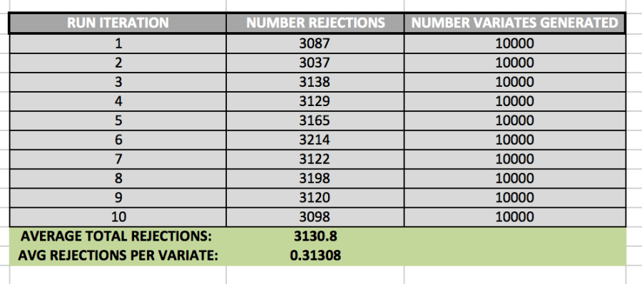
While generating 10,000 variates, the algorithm created 3130.8 rejections, on average. This means that, generally, there was about 1 rejected variate for every 3 valid variates.
Polar-Coordinate Method
In the Polar-Coordinate method, we take advantage of trigonometric properties by generating random variables uniformly distributed over (0, 2pi), and then transforming them into rectangular coordinates. This method, called the Box-Muller Method more formally, is not computationally efficient, however, because it involves use of logs, sines, and cosines—all expensive operations on a CPU.
In order to perform this operation more efficiently, I’ve used the method outlined by Sheldon Ross, on page 83 of his book Simulation (5th Ed.).
Step 1: Generate random numbers, U1 and U2
Step 2: Set V1 = 2U1 – 1, V2 = 2U2 – 1, S = V12 + V22
Step 3: If S > 1, return to Step 1.
Step 4: Return the independent standard normal for two variables, X and Y:
Where:
X = sqrt(-2*log(S)/2) * V1,
Y = sqrt(-2*log(S)/S)*V2
Expectations
Prior to running the experiment, I expected the Inverse-Transform Method to generate the worst variables themselves, because it only uses an approximation of the Standard Normal CDF, not the CDF itself. I was a little nervous about using an approximation for a CDF with no closed form to generate my inverse function, thinking that while our inverse may deliver results that are more or less reasonable, the resulting data set wouldn’t pass more advanced statistical tests since we are presumably losing precision, through the approximation process. But that said, I also expected its time efficiency to be the best, because we are only calculating logarithm each time we call the inverse function, and this seems to be the only slow operation.
I expected that method 2, Accept/Reject generate the most accurate variables, mostly because of the convincing mathematical proofs describing its validity on pages 77 and 78 of Ross’s Simulation textbook. Intuitively, the proof for this method makes sense, so I expected its data set to look most like something that truly follows the Standard Normal Distribution. From a time efficiency standpoint however, I expected this algorithm to perform 2nd best, because I’m using a logarithm each time I generate an exponential random variable. And with 2 log calls for each run, it seems like this method would be relatively slow, under the assumption that Python’s log function is expensive. (Log calls are used here because we know that –logU is exponential with rate lambda=1. But we need exponential variables generated with rate 1 for each Y variable, Y1 and Y2.)
The Polar Coordinate Method is the most abstract for me, and so I had a hard time seeing exactly why it would generate Standard Normal Random variables, and because of this, I wasn’t sure what to expect of its data set. I took it on faith that it would generate the correct variables, but I didn’t fully understand why. Moreover, I also expected it to perform the worst from a runtime perspective because it involves the most expensive operations: Two Square Roots and Two Log calls for each successful run.
Histograms and Analysis
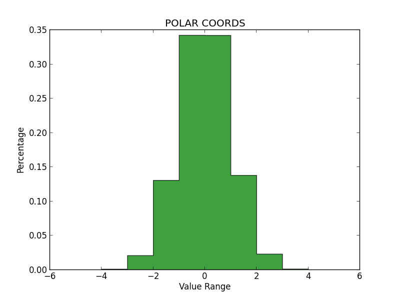
In order to determine whether each method produced qualitatively accurate data, I then plotted histograms for the numbers generated by each. All three histograms can be seen below. On my examination, it appears that the Inverse Transform yielded the least accurate representation, while the Polar Coordinate Method and Accept/Reject were much better, and about equal in validity.
Notably, the Inverse Transform method generated many values beyond the expected range of the Standard Normal (greater than 4.0 and less than -4.0). And while these values are possible, it seems like too many outliers—more than we would see in a true Standard Normal Distribution. Again, I think this is because we are using an approximation for the CDF, rather than the true Inverse of the CDF itself. I had some trouble getting these graphs to sit in-line, so please review the appendix to see them.
Chi-Squared Test
In order to determine wither the numbers generated may be from the Normal Distribution, I ran each method 10 times, and performed a Chi-Square test on each result. The data set can be seen in the tables within the appendix at the back of this document.
From this test, I was able to make the following determinations:
- Inverse Transform:
- N=10,000
- Avg Chi Sq: 2,806.719
- From 10 tests, each n=10,000
- Critical Value:749
- Result: REJECT Null Hypothesis
- Accept/Reject
- N=10,000
- Avg Chi Sq: 10,025.226
- From 10 tests, each n=10,000
- Critical Value: 10,233.749
- Result: ACCEPT Null Hypothesis
- Accept/Reject
- N=10,000
- Avg Chi Sq: 9,963.320
- From 10 tests, each n=10,000
- Critical Value: 10,233.749
- Result: ACCEPT Null Hypothesis
Runtime Analysis
Again, I ran each method 10 times to collect a sample of data with which to analyze runtime.
The average runtimes from 10 tests with n=10,000 were:
- Inverse Transform: -6.60E-06 seconds
- Accept/Reject: -5.72E-06 seconds
- Polar Coordinates: –63E-06 seconds
This result was indeed surprising. I had expected the Polar Coordinates method to perform the worst, and it did—but only by a very small margin. Moreover, I had expected Inverse Transform to perform the best, and it was only fractions of a microsecond (or nanosecond?) faster than Polar Coordinates on average. I did not expected Accept/Reject to perform so well, but it was by far the fastest overall.
Conclusion
Given these results, I would recommend the Accept/Reject method for anyone who needs to generate Standard Normal Random Variables in Python (at least using my same implementations).
Accept/Reject not only passed the Chi-Square test at the 95% significance level, it also was by far the fastest of the three algorithms. It is roughly comparable to Polar Coordinates on the quality of variables generated, and it beats everything else on speed.
APPENDIX – FIGURES:
Fig 1.1 – Inverse Transform Method Histogram

Fig 1.2 – Polar Coordinates Method HistogramFig 1.3 – Accept/Reject Method Histogram
DATA ANALYSIS TABLES
| INVERSE TRANSFORM | ||||
| RUN ITERATION | CHI SQ | CRIT VALUE, ALPHA=0.05 | NULL HYPOTHESIS | TIME |
| 1 | 29076.10305 | 10233.7489 | REJECT | -7.87E-06 |
| 2 | 28786.13727 | 10233.7489 | REJECT | -5.96E-06 |
| 3 | 29238.94032 | 10233.7489 | REJECT | -6.20E-06 |
| 4 | 27528.91629 | 10233.7489 | REJECT | -8.11E-06 |
| 5 | 28302.76943 | 10233.7489 | REJECT | -5.96E-06 |
| 6 | 28465.05791 | 10233.7489 | REJECT | -5.96E-06 |
| 7 | 28742.14355 | 10233.7489 | REJECT | -6.91E-06 |
| 8 | 29462.56461 | 10233.7489 | REJECT | -5.96E-06 |
| 9 | 28164.87435 | 10233.7489 | REJECT | -6.20E-06 |
| 10 | 28319.68265 | 10233.7489 | REJECT | -6.91E-06 |
| AVG CHI SQ: | 28608.71894 | 10233.7489 | REJECT | |
| AVG TIME SPENT: | -6.60E-06 |
| ACCEPT/REJECT | ||||
| RUN ITERATION | CHI SQ | CRIT VALUE, ALPHA=0.05 | NULL HYPOTHESIS | TIME |
| 1 | 9923.579322 | 10233.7489 | FAIL TO REJECT | -6.91E-06 |
| 2 | 10111.60494 | 10233.7489 | FAIL TO REJECT | -5.01E-06 |
| 3 | 9958.916425 | 10233.7489 | FAIL TO REJECT | -5.01E-06 |
| 4 | 10095.8972 | 10233.7489 | FAIL TO REJECT | -7.15E-06 |
| 5 | 10081.61377 | 10233.7489 | FAIL TO REJECT | -5.96E-06 |
| 6 | 10050.33609 | 10233.7489 | FAIL TO REJECT | -5.01E-06 |
| 7 | 9952.663806 | 10233.7489 | FAIL TO REJECT | -5.01E-06 |
| 8 | 10008.1 | 10233.7489 | FAIL TO REJECT | -5.01E-06 |
| 9 | 9953.795163 | 10233.7489 | FAIL TO REJECT | -6.20E-06 |
| 10 | 10115.71883 | 10233.7489 | FAIL TO REJECT | -5.96E-06 |
| AVG CHI SQ: | 10025.22255 | 10233.7489 | FAIL TO REJECT | |
| AVG TIME SPENT: | -5.72E-06 |
| POLAR COORDINATES | ||||
| RUN ITERATION | CHI SQ | CRIT VALUE, ALPHA=0.05 | NULL HYPOTHESIS | TIME |
| 1 | 9765.748259 | 10233.7489 | FAIL TO REJECT | -5.96E-06 |
| 2 | 9841.898918 | 10233.7489 | FAIL TO REJECT | -4.05E-06 |
| 3 | 10014.11641 | 10233.7489 | FAIL TO REJECT | -5.96E-06 |
| 4 | 10154.0752 | 10233.7489 | FAIL TO REJECT | -7.15E-06 |
| 5 | 10081.61377 | 10233.7489 | FAIL TO REJECT | -7.15E-06 |
| 6 | 9964.385625 | 10233.7489 | FAIL TO REJECT | -5.96E-06 |
| 7 | 9860.196443 | 10233.7489 | FAIL TO REJECT | -4.05E-06 |
| 8 | 9903.479938 | 10233.7489 | FAIL TO REJECT | -1.38E-05 |
| 9 | 10037.27323 | 10233.7489 | FAIL TO REJECT | -7.15E-06 |
| 10 | 10010.40893 | 10233.7489 | FAIL TO REJECT | -5.01E-06 |
| AVG CHI SQ: | 9963.319674 | 10233.7489 | FAIL TO REJECT | |
| AVG TIME SPENT: | -6.63E-06 |
| ACCEPT / REJECT – REJECTIONS | ||
| RUN ITERATION | NUMBER REJECTIONS | NUMBER VARIATES GENERATED |
| 1 | 3087 | 10000 |
| 2 | 3037 | 10000 |
| 3 | 3138 | 10000 |
| 4 | 3129 | 10000 |
| 5 | 3165 | 10000 |
| 6 | 3214 | 10000 |
| 7 | 3122 | 10000 |
| 8 | 3198 | 10000 |
| 9 | 3120 | 10000 |
| 10 | 3098 | 10000 |
| AVERAGE TOTAL REJECTIONS: | 3130.8 | |
| AVG REJECTIONS PER VARIATE: | 0.31308 |

You must be logged in to post a comment.