Being someone who programs but also values my sanity and doesn’t work on anything as important as mission control systems, the #1 way that I evaluate how much I like a programming language is usability: do I enjoy using it?
But I’ve never found something that seemed completely intuitive to me.
And the worst of everything was Haskell. I tried learning it a few times because–in theory–it seems so damn cool.
But actually using for a real project seemed kind of futile. It feels like you’re literally fighting with the compiler sometimes, and the syntax is extremely foreign to someone who came of age using C family languages. At least when you first start. There are so many times when I’m going through exercises and think — yeah I know exactly how to do that: I’ll hash this, then run so and so’s algorithm on it… but then you can’t even get I/O because that’s a Monad or something.
Today, I was going through yet *another* Haskell book, Chris Allen’s Programming Haskell From First Principles, and I finally did an exercise that made it click: Binary Tree Traversals.
Here’s a Binary Tree data structure:
This file contains hidden or bidirectional Unicode text that may be interpreted or compiled differently than what appears below. To review, open the file in an editor that reveals hidden Unicode characters. Learn more about bidirectional Unicode characters
This file contains hidden or bidirectional Unicode text that may be interpreted or compiled differently than what appears below. To review, open the file in an editor that reveals hidden Unicode characters. Learn more about bidirectional Unicode characters
You don’t need to make stacks and queues or keep track of what’s been visited. Instead it’s like drawing a picture. You can pattern match everything, literally placing the values where you want them to *visually* end up in the resulting list, and it gets built up through the natural recursion. Each recursive call builds its own sublist, and then–only when that recursion is finished–the resulting list gets added into the bigger one which is eventually returned. The simplicity is kind of mind blowing.
But what’s interesting to me is that getting to the point where this makes sense takes so long. So much frustration. And then out of nowhere, it’s all so simple. Haskell is the only programming language I’ve ever learned where I felt that way.
Most of the others have what you might call linear learning curves. Some are steeper than others, but you see results immediately. With Haskell, you read three books and still don’t totally understand what the hell is going on. Then, you’re doing a random exercise one day, and not only do you “get” it, but you realize it’s amazingly simple. I don’t know if that’s good usability. But it’s a unique experience, and one that’s very satisfying.
So I guess what I’m saying is this:Don’t give up if you’re trying to learn this stuff. When you least expect it, everything will click. And then you’ll wonder why it took so long.
How I think about art, and a proposal for how we might one day measure and quantify art, from the POV of computer science. Also: a novel strategy for making winning investments in the art world
Art and Use-value
I highly doubt this view is original, but I’ve never seen anyone else present it, and I feel like it’s the most practically useful way for me to view:
The purpose of art
What makes some artworks more successful (or better) than others
I’m less interested in giving a philosophical background for why someone might be interested these questions (there’s already enough written on that), so I’m going to jump right in.
I’ll present this as a very simple (and very informal) logical argument. I don’t think it’s ‘right’ in the sense that things are absolutely right or wrong (and honestly, I don’t care), but I think it’s an interesting and constructive way to view art (a subject I’ve always loved and been interested in). And moreover, as a student of computer science, I also believe this view offers a novel way to measure things we generally think of as intangible and subjective, such as ‘the quality of of an artwork’.
DISCLAIMER: Except maybe in advertising agencies, the value of art has always been subjective, and it will hopefully remain that way–but I still wonder, maybe just as an intellectual exercise: is there a way that we might quantify art in terms of a specific use-value? I think there is. And details are below.
Propositions
The Purpose of art
1) The purpose of art is to transmit to emotional information
How to judge the quality of art
2) If the purpose of art is to transmit emotional information, then artwork that transfers more emotional information can be said to be of ‘higher quality’
3) Since large artworks (think: a novel of 3,000 pages, or wall-sized painting) have more opportunity to transfer emotional information than small artworks (think: a 10 page short story, or 5x5inch painting) —> THEN: the best way to measure the quality of an artwork is not just the *amount* of emotional information it transfers, but how much emotional information it transfers given its size.
That is, what we really want to measure is emotional information density, emotional entropy.
And specifically: the more emotion that gets packed into an artwork, the better.
Here’s a graphic I made using Balsamiq. It’s crude and kind of sarcastic, but you get the point:
Click for larger version
Art as compression
4) In computer science packaging information into a smaller file format so that it can be more easily transferred is called compression. There are many compression algorithms, and some are better than others at different tasks. The goal of compression, very simply, is this: Package as much information as you can into the smallest file size possible. Then transfer it to another person. That person de-compresses the compressed file and gets ALL of the information, even though it was transferred in a much smaller package.
My suggestion is this: We can think of an artwork as the compressed file. We can think of the emotional content the artist is trying to convey as the compressed data. And we can think of the an artist’s technique or creative strategies as his compression algorithm. The better the algorithm, the more the data gets compressed, and the more information we can transfer in less space.
The role of artists
5) Following this analogy, I suggest that: the role of artists is to put as much emotion as possible into their package (the artwork) so that these emotions can be experienced across time and space. And the more emotional information an artist is able to transfer, the better the artwork. The goal of art, really is information transfer, a very specific kind of communication. We want to make others feel a certain way: We want to make others know that someone is there for them. That we all feel the same emotions sometimes. That there can be transcendence, that there can be an end to metaphysical sadness—this and so much more. All of it can be possible, and there’s a role for all of it.
What it means practically
6) For artists: Think very carefully about the emotional content you intend to transfer to others. If your goal is to make others feel specific emotions, then what emotions do you want to share, is there a sort of responsibility that comes with being a tremendously gifted artist? (I mean, I wouldn’t really want to paint things that made everyone feel desolation and sadness, rather than profundity, transcendence and stillness.)
7) For computer scientists: Using this heuristic, maybe it’s possible to evaluate a body of work from different historical artists and determine the ‘most artistic’ of them all. For instance: take all the paintings in a given museum, and ask visitors to rate the amount of emotion they experience while looking at them (say on a 1-100 scale). Then, normalize this data based on the size of the artwork, and see which painting has the highest ‘emotional entropy’: The most emotional content given its size. Is this the greatest, or ‘most artistic’ artwork in museum? Either way, it’s hard to argue that it’s not the most successful.
How to make money from it =)
(see, I wasn’t just BSing about use-value)
This gets even more interesting once we think: Can we tie emotional entropy to historic auction prices? If there’s a relationship, and we can establish that, couldn’t we use this relationship to identify the contemporary artworks (even from relatively young or unknown artists) that will one day sell for the most money? And if so, shouldn’t we start buying them all immediately? There’s a business idea there that’s free for the taking… I’m being somewhat sarcastic, but in all seriousness, I think it would be very interesting to examine this data and try, even as an experiment. So if you’re similarly interested, feel free to contact me.
I needed to generate Standard Normal Random Variates for a simulation I’m programming, and I wanted to see which method would be best to use. There are a few options, but generally you need to experiment to know for sure which will work best in your situation.
I decided to do this in Python, and to share my code + experimentation process and recommendations/reasoning.
Hoping this can save someone else some time later. If you need to do the same for your own simulation, or any other reason, hopefully this solves some of your problems, helps you understand what’s going on under the hood, and just makes life easier.
I used Python to algorithmically generate random variates that follow the Standard Normal distribution according to three different methods. For all methods, 10,000 valid random variables were generated in each algorithm’s run, in order to maintain consistency for later effectiveness comparisons. The methods tested were:
The Inverse Transform Method
The Accept/Reject Method
The Polar-Coordinates Method
In the following paragraphs, I will briefly outline the implementation decisions made to generate Standard Normal random variates according to each method. I will then analyze the results, compare them, and issue my own recommendation on which method to use going forward, informed by the data gathered in this experiment.
Inverse Transform
The Inverse Transform Method works by finding the inverse of the CDF for a given probability distribution (F-1(X)), then feeding random numbers generated from U[0,1) into that inverse function. This will yield randomly generated variables within the range of our desired probability distribution.
However, this method is problematic for the Standard Normal Distribution, because there is no closed form for its CDF, and hence we cannot calculate its exact inverse. Because of this, I chose to use Bowling’s closed-form approximation of the Standard Normal CDF, which was developed in 2009: Pr(Z <= z) = 1 / [1 + e^(-1.702z)].
Despite being only an approximation, Bowling’s closed form CDF function is mathematically close enough to generate reasonable random variates. Beyond that, this function is simple. The hardest part was calculating the inverse, which was actually done with help from Wolfram Alpha. Once an inverse was obtained, implementation was straightforward and can be seen in the code attached, within the method @inverse_transform().
Accept/Reject
The Accept/Reject method for random variate is more complex, and it can be implemented a few different ways. I chose to use the method outlined by Sheldon Ross in his book Simulation (Fifth Edition), on page 78.
The procedure, and a snippet of the core code used, are both presented in-line below, as an illustration:
This file contains hidden or bidirectional Unicode text that may be interpreted or compiled differently than what appears below. To review, open the file in an editor that reveals hidden Unicode characters. Learn more about bidirectional Unicode characters
To note: Our Y1 and Y2 values are seeded with variates generated by the exponential distribution, with lambda=1. In much of the literature on the Accept/Reject method, this function is called “g(x)”, and for this example we used the exponential distribution.
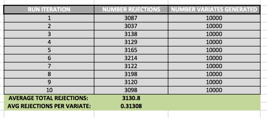
It is also important to keep track of how many rejections we get while using the Accept/Reject method. In order to determine the average number of rejections, I ran the algorithm 10 times. The data set it created is shown below:
While generating 10,000 variates, the algorithm created 3130.8 rejections, on average. This means that, generally, there was about 1 rejected variate for every 3 valid variates.
Polar-Coordinate Method
In the Polar-Coordinate method, we take advantage of trigonometric properties by generating random variables uniformly distributed over (0, 2pi), and then transforming them into rectangular coordinates. This method, called the Box-Muller Method more formally, is not computationally efficient, however, because it involves use of logs, sines, and cosines—all expensive operations on a CPU.
In order to perform this operation more efficiently, I’ve used the method outlined by Sheldon Ross, on page 83 of his book Simulation (5th Ed.).
Step 1: Generate random numbers, U1 and U2
Step 2: Set V1 = 2U1 – 1, V2 = 2U2 – 1, S = V12 + V22
Step 3: If S > 1, return to Step 1.
Step 4: Return the independent standard normal for two variables, X and Y:
Where:
X = sqrt(-2*log(S)/2) * V1,
Y = sqrt(-2*log(S)/S)*V2
Expectations
Prior to running the experiment, I expected the Inverse-Transform Method to generate the worst variables themselves, because it only uses an approximation of the Standard Normal CDF, not the CDF itself. I was a little nervous about using an approximation for a CDF with no closed form to generate my inverse function, thinking that while our inverse may deliver results that are more or less reasonable, the resulting data set wouldn’t pass more advanced statistical tests since we are presumably losing precision, through the approximation process. But that said, I also expected its time efficiency to be the best, because we are only calculating logarithm each time we call the inverse function, and this seems to be the only slow operation.
I expected that method 2, Accept/Reject generate the most accurate variables, mostly because of the convincing mathematical proofs describing its validity on pages 77 and 78 of Ross’s Simulation textbook. Intuitively, the proof for this method makes sense, so I expected its data set to look most like something that truly follows the Standard Normal Distribution. From a time efficiency standpoint however, I expected this algorithm to perform 2nd best, because I’m using a logarithm each time I generate an exponential random variable. And with 2 log calls for each run, it seems like this method would be relatively slow, under the assumption that Python’s log function is expensive. (Log calls are used here because we know that –logU is exponential with rate lambda=1. But we need exponential variables generated with rate 1 for each Y variable, Y1 and Y2.)
The Polar Coordinate Method is the most abstract for me, and so I had a hard time seeing exactly why it would generate Standard Normal Random variables, and because of this, I wasn’t sure what to expect of its data set. I took it on faith that it would generate the correct variables, but I didn’t fully understand why. Moreover, I also expected it to perform the worst from a runtime perspective because it involves the most expensive operations: Two Square Roots and Two Log calls for each successful run.
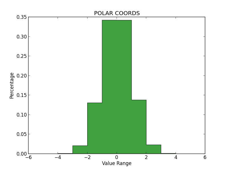
Histograms and Analysis
In order to determine whether each method produced qualitatively accurate data, I then plotted histograms for the numbers generated by each. All three histograms can be seen below. On my examination, it appears that the Inverse Transform yielded the least accurate representation, while the Polar Coordinate Method and Accept/Reject were much better, and about equal in validity.
Notably, the Inverse Transform method generated many values beyond the expected range of the Standard Normal (greater than 4.0 and less than -4.0). And while these values are possible, it seems like too many outliers—more than we would see in a true Standard Normal Distribution. Again, I think this is because we are using an approximation for the CDF, rather than the true Inverse of the CDF itself. I had some trouble getting these graphs to sit in-line, so please review the appendix to see them.
Chi-Squared Test
In order to determine wither the numbers generated may be from the Normal Distribution, I ran each method 10 times, and performed a Chi-Square test on each result. The data set can be seen in the tables within the appendix at the back of this document.
From this test, I was able to make the following determinations:
Inverse Transform:
N=10,000
Avg Chi Sq: 2,806.719
From 10 tests, each n=10,000
Critical Value:749
Result: REJECT Null Hypothesis
Accept/Reject
N=10,000
Avg Chi Sq: 10,025.226
From 10 tests, each n=10,000
Critical Value: 10,233.749
Result: ACCEPT Null Hypothesis
Accept/Reject
N=10,000
Avg Chi Sq: 9,963.320
From 10 tests, each n=10,000
Critical Value: 10,233.749
Result: ACCEPT Null Hypothesis
Runtime Analysis
Again, I ran each method 10 times to collect a sample of data with which to analyze runtime.
The average runtimes from 10 tests with n=10,000 were:
Inverse Transform: -6.60E-06 seconds
Accept/Reject: -5.72E-06 seconds
Polar Coordinates: –63E-06 seconds
This result was indeed surprising. I had expected the Polar Coordinates method to perform the worst, and it did—but only by a very small margin. Moreover, I had expected Inverse Transform to perform the best, and it was only fractions of a microsecond (or nanosecond?) faster than Polar Coordinates on average. I did not expected Accept/Reject to perform so well, but it was by far the fastest overall.
Conclusion
Given these results, I would recommend the Accept/Reject method for anyone who needs to generate Standard Normal Random Variables in Python (at least using my same implementations).
Accept/Reject not only passed the Chi-Square test at the 95% significance level, it also was by far the fastest of the three algorithms. It is roughly comparable to Polar Coordinates on the quality of variables generated, and it beats everything else on speed.
This file contains hidden or bidirectional Unicode text that may be interpreted or compiled differently than what appears below. To review, open the file in an editor that reveals hidden Unicode characters. Learn more about bidirectional Unicode characters
I generated some random numbers with a few different generators, some of which I made, and also used the one provided directly by Python. I wanted to see what the best option is for generating random numbers in a few simulations I’m doing.
It’s commented and can be run by simply invoking Python with: “python lcg.py”
I tried to explain what I was doing at each step to make this clear even for the comparatively un-initiated to the more esoteric statistics at play here, which aren’t totally necessary to know, and really will just be an impediment to __getting_started_now__. I wanted to share something so that people who are practically-minded like me can just jump in, start messing around, and know what to expect. So hopefully with just this code (full repo linked below) and the information presented here, you can start messing around with random number generators if you need to for any reason. (Most common reason would be to seed random variates in a simulation.)
My main goal in posting this is to give anyone with an interest in generating randomness an easy entry into it–with working code for these sort of generators, as it’s somewhat hard to find online, and the details can be a bit opaque, without clear examples of what to expect when you’re testing. So ideally, this will be the total package. Probably not, but hey, giving it a try. If for some reason you need help, feel free to contact me.
Random Number Generation
Generating truly random numbers is a longstanding problem in math, statistics, and computer science. True randomness requires true entropy, and in many applications—such as generating very large sets of random numbers very quickly—sufficient “true” entropy is difficult or impractical to obtain. (Often, it needs to come from the physical environment, sources such as radioactive decay, etc.) So, instead, we look to algorithmic random numbergenerators for help.
Algorithmically generated random numbers will never be “truly” random precisely because they are generated with a repeatable algorithmic formula. But for purposes such as simulating random events – these “Pseudo-random” numbers can be sufficient. These algorithmic generators take a “seed value” from the environment, or from a user, and use this seed as a variable in their formula to generate as many random-like numbers as a user would like.
Naturally, some of these algorithms are better than others, and hundreds (if not thousands, or more) of them have been designed over the years. The output is always deterministic, and never “truly” random, but the ideal goal is to approximate randomness by generating numbers which:
Are uniformly distributed on the range of [0,1)
Are statistically independent of each other
(That is, the outcomes of any given sequence do not rely on previously generated numbers)
The best random number generators will pass statistical tests for both uniformity and independence. In this analysis, we will subject three different random number generation algorithms to series of statistical tests and compare the outcomes.
The algorithms we will test are:
Python’s Built-In Random Number Generator
This algorithm is called the “Mersenne Twister”, implementation details are available at: Python Docs for Random
Seed value: 123456789
A Linear Congruential Generator
Seed value: 123456789
a=101427
c=21
m=216
A Linear Congruential Generator with RANDU initial settings
Seed value: 123456789
a=65539
c=0
m=231
The tests each algorithm will be subjected to are:
Uniformity tests
Chi-squared Test for Uniformity
Kolmogorov-Smirnov Test for Uniformity
Null hypothesis for BOTH tests: The numbers in our data set are uniformly distributed
Independence tests
Runs Test for Independence
Autocorrelation Test for Independence, (gap sizes: 2,3,5, and 5 will be used)
Null hypothesis for BOTH tests: The numbers in our data set are independent of each other
Test Result Summary & Quick Notes on Implementation
The exact implementation of each test can be viewed in the linked Python file named: “lcg.py”. The tests can be duplicated by anyone with Python installed on their system by running the command “python lcg.py”.
You can view the file directly on GitHub here: >> lcg.py <<
SUMMARY TABLE (2.1)
Algorithm
X2
TS/Result
KS TS/Result
Runs
TS/ Result
Autocorrelation
TS/Result
Mersenne Twister (PyRand)
9.754
Pass all
0.079213
Pass all
-1.6605
Reject at 0.8 and 0.9
Pass at 0.95
Gap=2: -1.089
Gap=3: -0.924
Gap=5: -0.559
Gap=50: -0.228
All Pass
LGC
6.288
Pass all
0.0537888
Pass all
0.5218
Pass all
Gap=2: 0.1753
Gap=3: -0.394
Gap=5: 0.872
Gap=50: 1.335
Reject at 0.8, Gap=50, others pass
LGC, w/ RANDU
12.336
Pass all
0.053579
Pass all
-0.2135
Pass all
Gap=2: -0.6591
Gap=3: -0.9311
Gap=5: 0.5788
Gap=50:-0.9093
All pass
The summary table above shows each algorithm tested, and which tests were passed or failed. More detailed output for each test and for each algorithm can be viewed in Tables 1.1 – 1.3 in the appendix to this document.
The Kolmogorov-Smirnov (or KS test) was run at the following levels of significance: .90, 0.95, 0.99. The formulas for the critical value at these significance levels were taken from table of A7 of Discrete-Event System Simulation by Jerry Banks and John S. Carson II. (Formulas for 0.80 could not be found, so I’ve used what was available.)
All other tests were run at the 0.80, 0.90., and 0.95 significance level.
Statistical Analysis and Expectations
Prior to generating the numbers for each test, I expected Python’s random function to perform the best of all three algorithms tested, mostly because it’s the library random function of one of the world’s most popular programming languages. (Which means: thousands and thousands of code repositories rely on it—many of which are used by commercial and mission critical programs.) But in fact, it performed the worst, failing the Runs Test at both the 0.80 and 0.90 level of significance. These failings are NOT statistically significant at the alpha=0.05 level, but it’s still surprising to see.
I expected the RANDU algorithm to perform the worst, and I thought it would perform especially badly on the autocorrelation test. This is because RANDU is known to have problems, outlined here. Specifically, it is known to produce values which fall along only a specific set of parallel planes (visualization in link above), which means the numbers should NOT be independent, when tested at the right gap lengths. It’s possible that the gap lengths I’ve tested simply missed any of these planes, and as a result—RANDU performed the best of all the algorithms. It’s the only algorithm that didn’t fail any statistical tests at all.
I anticipated the LGC function to perform 2nd best overall, and I was right about that—but the best and worst algorithm were the opposite of what I expected. Mostly, I thought that that Python’s random generator would be nearly perfect, RANDU would be badly flawed, and the LGC would be just okay. Really, the LGC performed admirably: The only test it failed was autocorrelation at the 0.80 confidence level, and that isn’t statistically significant by most measures.
Reviewing the data output into each .txt file directly, I don’t see any discernible patterns in the numbers themselves. And with 10,000 data points, there’s so much output to review that I can see why statistical measures are needed to effectively to determine what’s really going on in the data. It’s probably possible to find a few patterns, specifically related to runs and gap-sequences just by viewing the data directly, but tests are still needed to find out for sure.
With that said, I do think the testing done in this experiment is sufficient, because we have two tests for each measure that matters: 1) Uniformity; 2) Independence. The only improvement I would make for future tests is testing more gap-sequences, and starting them at different points. I’d do this mostly because I know that RANDU should fail gap-sequence tests given the right input, but there would be some trial and error involved in trying to find these sequences naively. So, sometimes, getting into math itself and working with proofs may still be the most effective method. Maybe sometime the old-fashioned way is still best.
TABLE 1.2 – Linear Congruential Generator (X0 = 123456789 )
Test Name
Sample Size
Confidence Level
Critical Value
Test Statistic Found
Result
Chi-Square
10,000
0.80
10118.8246
6.288
FAIL TO REJECT null
Chi-Square
10,000
0.90
10181.6616
6.288
FAIL TO REJECT null
Chi-Square
10,000
0.95
10233.7489
6.288
FAIL TO REJECT null
Kolmogorov-Smirnov
100
0.90
0.122
0.05378
FAIL TO REJECT null
Kolmogorov-Smirnov
100
0.95
0.136
0.05378
FAIL TO REJECT null
Kolmogorov-Smirnov
100
0.99
0.163
0.05378
FAIL TO REJECT null
Runs Test
10,000
0.80
1.282
0.521889
FAIL TO REJECT null
Runs Test
10,000
0.90
1.645
0.521889
FAIL TO REJECT null
Runs Test
10,000
0.95
1.96
0.521889
FAIL TO REJECT null
Autocorrelation,
GapSize=2
10,000
0.80
1.282
0.175377
FAIL TO REJECT null
Autocorrelation,
GapSize=2
10,000
0.90
1.645
0.1753777
FAIL TO REJECT null
Autocorrelation,
GapSize=2
10,000
0.95
1.96
0.1753777
FAIL TO REJECT null
Autocorrelation,
GapSize=3
10,000
0.8
1.282
-0.39487
FAIL TO REJECT null
Autocorrelation,
GapSize=3
10,000
0.9
1.645
-0.39487
FAIL TO REJECT null
Autocorrelation,
GapSize=3
10,000
0.95
1.96
-0.39487
FAIL TO REJECT null
Autocorrelation,
GapSize=5
10,000
0.8
1.282
0.872668
FAIL TO REJECT null
Autocorrelation,
GapSize=5
10,000
0.9
1.645
0.872668
FAIL TO REJECT null
Autocorrelation,
GapSize=5
10,000
0.95
1.96
0.872668
FAIL TO REJECT
null
Autocorrelation,
GapSize=50
10,000
0.8
1.282
1.3352
REJECT null
Autocorrelation,
GapSize=50
10,000
0.9
1.645
1.3352
FAIL TO REJECT null
Autocorrelation,
GapSize=50
10,000
0.95
1.96
1.3352
FAIL TO REJECT null
Test Name
Sample Size
Confidence Level
Critical Value
Test Statistic Found
Result
END TABLE 1.2
TABLE 1.3 – Linear Congruential Generator with RANDU initial settings
Need to download data from Yahoo Finance using Java?
I wrote this utility as part of larger project and realized it could be re-used. Needed a name, so calling it Y-Financier. Posting here in case anyone else can benefit.
Add the Y-Financier Class to your project (copy/paste is fine)
Create an instance of the Y-Financier class
Pass your class instance the Ticker Symbol of the stock you’re interested in as the first argument (I.e. — “AAPL” for Apple)
Pass the name of the file where you’d like to store your data as the second argument
Call the #downloadFile method from your instance
And you’re done.
Notes:
This program will always download the most recently available full day’s earnings report. These are usually posted after 8 or 9pm Eastern Time. If you run this program before 8 or 9pm ET, you’ll be downloading yesterday’s report. (Getting real-time stock market data will require a different solution.)
This program will always overwrite the previously downloaded file. That setting can be changed, but it will need to be done in the source.
I’m using Ben Noland’s implementation for the #saveURL function, found here.
A concrete example of how to use the class can be found in my Main.java file.
If you’re using Java on a similar project, save your time. Y-Financier will make it money. (hopefully.)


You must be logged in to post a comment.